Variational Quantum Eigensolver #

Contents

Variational Quantum Eigensolver

Background #

It might be surprising that we have gone so far with the structure of quantum mechanics without looking at many of the systems the theory was developed to handle. So, lets spend a small amount of time looking at the classical systems that you would treat in an undergraduate quantum mechanics class, and start with the Schrodinger equation

\[\begin{gather*} \hat{H}\ket{\psi} = i\hbar\partial_t\ket{\psi} \end{gather*}\]

Where the \(\hat{H}\) is an operator that corresponds with the classical Hamiltonian following the following quantization rules for a position basis.

\[ \hat{p} = -i\hbar\partial_x,\ \hat{x} = x \]

So, in cases where \(\hat{H}\) is not time-dependent, we can use separation of variables to write the Schrodinger equation as

\[ \hat{H}\ket{\psi} = E\ket{\psi},\ \ket{\psi_t} = e^{\hbar tE/i}\ket{\psi} \]

Where

\[ \hat{H} = \frac{\hat{p}^2}{2m}+\hat{V}(x) \]

Now, the main task of most intro quantum mechanics courses is determining \(\psi(x,t)\) for any given potential.

Hydrogen Atom #

A useful example of such a problem is the hydrogen atom, for reasons that we will see later. Here, we have a central potential namely,

\[ \hat{V}(x) = -\frac{Z}{r} \]

Now since the nucleus is rather heavy compared to the electron mass, it is as if the nucleus is stationary. Then the electron wave function is described by the following differential equation.

\[ \left(\frac{\hbar}{2m}\nabla^2+\frac{Ze^2}{r}\right)\psi(\vec{x}) = -E\psi(\vec{x}) \]

This can be broken into a radial and angular component \(\psi(r,\theta,\phi) = R(r)Y_l^m(\theta,\phi)\) with the following differential equations.

\[\begin{gather*} \frac{d^2}{d\phi^2}M(\phi) + m^2M(\phi) = 0\\ -\frac{\hbar^2}{2m}\left[(1-u^2)\frac{d^2}{du^2}-2u\frac{d}{du}+\left(l(l+1)-\frac{m^2}{1-u^2}\right)\right]P_l^m(u) = 0\\ -\frac{\hbar^2}{2m}\left[\frac{d^2}{dr^2}+\frac{l(l+1)}{r^2}\right]R(r)-\frac{Ze^2}{r}R(r) = ER(r) \end{gather*}\]

The combined angular solutions give the \(Y_l^m(\theta,\phi)\) spherical harmonics, while the radial solution is more complicated.

\[ R(r) \propto e^{-\frac{r}{a_0 n}}\mathcal{L}_{2l+1}^{n+1}\left(2r/na_0\right) \]

where \(a_0\) is the Bohr radius. The corresponding energy levels come directly from this equation giving us.

\[ E = -\frac{me^2}{2\hbar^2n^2},\ n\in \mathbb{N},\ l \in [0, n]\cap \mathbb{Z},\ m\in [-l, l]\cap \mathbb{Z} \]

Variational Method #

In many situations the above analysis is too complex to analyze and as physicists, we look to approximation to fill in the gaps. In many cases, this is done via perturbation theory where we build a real system up by perturbing a system that is exactly solvable. For example, to fully tackle the Hydrogen atom we must introduce perturbations for relativistic corrections, and interactions between the spin and orbit angular momentums. However, there are other classes of problems where the system has no simplified version that is exactly solvable, or when such a system would need to be perturbed to such an extent that perturbative corrections are no longer valid. In many of these cases, we look at these problems through the lens of the method of variation of parameters.

This method works by supposing the form of the ground state solution using known properties of the system, and symmetries, let \(\ket{\alpha}\) be our trial function with parameter \(\alpha\). If we consider the expectation value of the Hamiltonian, we find

\[ \langle H\rangle = E_\alpha = \bra{\alpha}H\ket{\alpha} \]

This is clearly the energy for if our proposed ground state wave function, since if \(\ket{\alpha} = \ket{n = 0}\), this is just the ground state energy. We show that this expectation value will always be larger than the ground-state energy. Taking the above statement, we insert a complete basis set

\[ E_\alpha = \sum_n\braket{\alpha|n}\bra{n}H\ket{\alpha} = \sum_n|\braket{\alpha|n}|^2E_n \]

Since the modulus squared of the matrix elements will always be positive definite, \(E_\alpha\geq E_0\). So, for the best approximation, we can minimize \(E_\alpha\) by variation of the parameter \(\alpha\).

Helium Atom #

To see how this works, let’s consider the Helium atom. Here we have two electrons orbiting a central unmoving nucleus. This could be explained by the following Hamiltonian

\[ H = -\frac{\hbar^2}{2m}\left(\nabla^2_1+\nabla^2_2\right)-Ze^2\left(\frac{2}{r_2}+\frac{2}{r_2}-\frac{1}{|\vec{r_1}-\vec{r_2}|}\right) \]

For a test function, let’s suppose

\[ \phi(\vec{r}_1,\vec{r}_2) = \frac{1}{\pi a^3}e^{-(r_1+r_2)/a} \]

Then by the method described above,

\[ E(a) = 2E_H(Z'^2-2(Z-5/16)Z') \]

Where \(Z' = a_0/a\), and \(E_H=13.6\)eV is the ground state energy of the hydrogen atom. Minimizing this as a function of \(Z'\) gives

\[ E_{var} = 25/128 E_H = 2.64\mathrm{eV} \]

The Variational Quantum Eigensolver #

The main goal of the Variational Quantum Eigensolver (VQE) is to find a way to implement this variational method on a quantum computer. This can be done by translating the ansatz wave function into our quantum computation terminology. We define our ansatz wavefunction as a general unitary operation \(U(\bf{\theta})\) on the initial state of \(N\) qbits, where \(\bf{\theta}\) is the set of parameters defining the operation. Then we can write down the variational method as follows

\[ E_{VQE} = min_\theta\bra{\bf{0}}U^\dagger HU\ket{\bf{0}}, \]

where for simplicity of notation, \(\ket{\bf{0}} = \ket{0}^{\otimes N}\). The output of this operation is will be some \(E(\bf{\theta})\) function called the cost function. The goal of the algorithm is to minimise the cost function quickly and efficiently by leveraging a quantum computer paired with a classical computer. This is done by re defining the hamiltonian as some equivelent set of rotations of individual qbits, and then dotting these rotated qbits to an input state. Then on a classical computer, the energy expectation values is calculated using our known initial guess \(U(\bf{\theta})\ket{\bf{0}}\) and our redefined Hamiltonian. This is used to define a new set of parameters \(\bf{\theta}\) that act as our new guess to start the process over again. This process is outlined in Fig.1.

**Fig.1.** The VQE Pipeline taken from Figure 1 in the paper The Variational Quantum Eigensolver: A review of methods and best practices.

Now there are some strange ideas that where thrown around when it comes to the Hamiltonian of the system being expressed as a unitary operation on qbits, and the exact state after the rotation being calculated. We know that measurements of quantum systems offer only a 1 or a 0, destroying the state in the process. Although we can use weak measurements to reduce the information we get while preserving aspects of the state, this is not what is happening. To get a feel for how this is done, let’s walk through the general process by which the Hamiltonian is constructed, our basis function is chosen, and the quantum computer operates on the state.

Pre Processing #

In the pre-processing step, we use a classical computer to build a problem that the quantum computer can solve. This means that we must choose a Hamiltonian representation, determine a strategy for building the initial state, and use these to build the quantum circuit. For simplicity, and connection to research that has been done, we will use the many body molecular Hamiltonian as an example.

Hamiltonian Construction #

There are two main schools of thought on the Hamiltonian. Either, we choose to use first quantization which has shown promise in scalability or the more prominent second quantization. Since it is more prominent and what Qiskit Nature uses, we will discuss second quantization.

Second quantization comes from turning the wave function into an operator, and as such, the wave function must now abide by the symmetry of the particles. In the case of electronic structure, we must use fermionic operators that encode their antisymmetric properties. To see how this is done, take the Many body electronic structure Hamiltonian.

\[ H = - \sum_I \frac{\nabla_{R_I}^2}{2M_I} - \sum_i \frac{\nabla_{r_i}^2}{2} - \sum_{I,i} \frac{Z_I}{|R_I-r_i|} + \sum_{i,j>i} \frac{1}{|r_i-r_j|} + \sum_{I,J>I} \frac{Z_I Z_J }{|R_I-R_J|} \]

Where, \(R_I\) is the position of nucleus \(I\), and \(r_i\) the position of electron \(i\). In a Born-Oppenheimer approximation, we treat the nuclear centers as stationary points of attraction for the electrons. As such the wave function can be separated into an electronic and nuclear part. To define the wave function, we use the fermionic creation and annihilation operators, \(a^\dagger_i\), and \(a_j\). With these operators, we can write the Hamiltonian as

\[ H = h_{ij}a^\dagger_i a^\dagger + \frac{1}{2}h_{ijkl}a^\dagger_i a^\dagger_j a_k a_l \]

with implied summation over repeated indices. These values \(h_{ij}\) and \(h_{ijkl}\) correspond to the integrals

\[ h_{ij} = \int d\bf{\sigma}\ \phi_i^*(\bf{\sigma})\left(\frac{\nabla_{r}^2}{2}-\sum_{I} \frac{Z_I}{|R_I-r|}\right)\phi_j(\bf{\sigma}) \]

\[ h_{ijkl} = \int d\bf{\sigma}_1 d\bf{\sigma}_2\ \frac{\phi_i^*(\bf{\sigma}_1)\phi_j^*(\bf{\sigma}_2)\phi_k(\bf{\sigma}_2)\phi_l(\bf{\sigma}_1)}{|\bf{r}_1-\bf{r}_2|} \]

where \(\bf{\sigma}\) includes the spin and spatial degrees of freedom of the basis function \(\phi(\sigma)\). Our choice in basis set is rather unimportant, but a popular one is the STO-NG basis set where the electron orbital is described by \(N\) Gaussians. Recall that these basis functions are like our Ansatz in a basic variation of parameters problem, and should be based on symmetries and properties of the system we are interested in. This is why molecular systems often use basis functions that are constructed from atomic linear combinations of atomic orbitals. A good explaination of this can be found from LibreTexts.

Now is a good time to ask how these second quantized operators preserve the fermionic antisymmetry. Well in the second quantization picture, the wave function we are discussing uses an occupation number basis, telling us how many particles occupy the first state, second state, and so on. These states are called Fock states

These operators have a particular algebraic structure spescific to fermions, this comes from their prior mentioned symmetry properties. In the case of fermionic operators, they must follow the commutation relation

\[ \{a_i,a^\dagger_j\} = \delta_{ij} \]

While standard \(2\times2\) hermitian matrices can be described by a linear combination of Pauli matrices and the identity, it is not clear that this algebraic structure can be preserved by this mapping. Fortunately, Jordan and Wigner showed an isomorphism between these fermionic operators and spin operators in a way that preserves the algebraic structure.

There are many such transformations that have been found after the [Jordan-Wignar transformation] each varying in one of the following three categories.

Number of Qbits: The number of qbits required to represent the electron wave function. In general, this is proportional to the number of sites that are being considered
Pauli weight: The maximum number of non-identity operators in any Pauli string produced by the transformation
Number of Pauli-strings: The number of Pauli strings produced by the mapping

In the JW transformation, these operators are expressed in the following way

\[ a^\dagger_i = \frac{1}{2}(X_i-iY_i)\bigotimes_i Z_{i<j}, \]

where the tensor product runs over all other states. Now, this transformation needs \(O(N)\) gates to construct any operator, so it is costly in the Number of gates needed metric. Though, some ansatzes algorithms can be used to deal with the anticommutation issues making this scale much nicer.

Another more complex algorithm is the Bravyi-Kitaev encoding which seeks to reduce the Pauli weight of the operators by encoding the parity and occupation numbers in qbits. There are some groups that have used this encoding to their advantage. For example, O’Malley uses this method to write their circuit for \(H_2\) using just 2 Qbits. From their paper, their effective Hamiltonian is writen as

\[ H = g_0I+g_1Z_0+g_2Z_1+g_3Z_0Z_1+g_4Y_0Y_1+g_5X_0X_1, \]

where the values \(g_i\) can be computed through some Hartree-Fock calculation and are dependent on the choice in basis functions. The exact method of arriving at this Hamiltonian is outlined by [O’Malley] in their appendex A. Using the values in their paper, we can do a quick diagonalization to determine the ground state energy of their system in this representation using pre computed values of \(g_i\) for STO-6G basis sets.

import numpy as np; from scipy.linalg import eig
np.set_printoptions(precision=4,suppress=True)
σ = np.array([[[1,0],[0,1]],[[0,1],[1,0]], [[0,-1j],[1j,0]],[[1,0],[0,-1]]])

g = np.array([-0.4804,+0.3435,-0.4347,+0.5716,+0.0910,+0.0910])
E_nuclear = 0.7055696146

H_electron = (g[0]*np.kron(σ[0],σ[0]) + #g0 * I
              g[1]*np.kron(σ[0],σ[3]) + #g1 * Z0
              g[2]*np.kron(σ[3],σ[0]) + #g2 * Z1
              g[3]*np.kron(σ[3],σ[3]) + #g3 * Z0Z1
              g[4]*np.kron(σ[2],σ[2]) + #g4 * Y0Y1
              g[5]*np.kron(σ[1],σ[1]))  # g5 * X0X1

E_electron = np.linalg.eigvalsh(H_electron) 

print(H_electron)

[[ 0.    +0.j  0.    +0.j  0.    +0.j  0.    +0.j]
 [ 0.    +0.j -1.8302+0.j  0.182 +0.j  0.    +0.j]
 [ 0.    +0.j  0.182 +0.j -0.2738+0.j  0.    +0.j]
 [ 0.    +0.j  0.    +0.j  0.    +0.j  0.1824+0.j]]

This is the non diagonalized Hamiltonian for just the electrons. Diagonalizing this computationally and adding the nuclerar repulsion energy gives the total interaction energy eigenvalues.

print(np.diag(E_electron+E_nuclear))
print("Diagonalization: {:+2.8}".format(E_electron[0] + E_nuclear))
print("Exact calculations: {:+2.8}".format(-1.1457416808))

[[-1.1456  0.      0.      0.    ]
 [ 0.      0.4528  0.      0.    ]
 [ 0.      0.      0.7056  0.    ]
 [ 0.      0.      0.      0.888 ]]
Diagonalization: -1.1456295
Exact calculations: -1.1457417

These values come from the summary done by Joshua Goings, where the exact calculation was computed using Gaussian 16 a computational chemestry software package.

Now, we want to run these calculations on a quantum computer and in theroy it makes sense that this should be possible. Each gate is some pauli gate so the operation can be done on a quantum computer; but again, the issue comes from getting the rotated state after it pases though the circuit. To answer this we still need to talk about building the ansatz and finish our pre processing discussion.

Ansatz Construction #

Now that we have our Hamiltonian expressed as a string of Pauli gates, we need to build our trial state. The overarching goal is to write a general state from some qbit registry. We know that an individual qbit can be expressed by the parameters \(\theta\), and \(\phi\) as

\[ \ket{\psi_\theta} = \cos(\theta/2)\ket{0}+e^{i\phi}\sin(\theta/2)\ket{1}. \]

But, this general state is simply generated from a rotation of \(\theta\) about the \(y\)-axis and a rotation of \(\phi\) about the \(z\)-axis on the Bloch sphere, i.e.,

\[ \ket{\psi_\theta} = R_y(\theta)R_z(\phi)\ket{0}. \]

After this combination of rotations is denoted \(U(\vec{\theta})\) where \(\vec{\theta}\) is the set of rotation parameters. This is the general process for generating an ansatz.

Now, while some algorithms converge well for any guess, the VQE is particular in that a poor choice in ansatz will lead to inaccurate results or poor convergences. There are two main catagories that must be considered when dealing with this algorithm

Expressibility:The expressibility of an ansatz describes its span across the unitary space of accessible states. In other words, this is a measure of how well the gates used to build the ansatz and the the ansatz can be used to manipulate the qbits into whatever state is needed for the algorithm to converge. This is usually quantified using the Haar measure by determining the distance between the unitaries that could be generated by the ansatz. For ansatz with extrodinarily large ansatz, the algorithm may become intractable as there are too many parameters to change. This is related to the barren plateau problem.
Trainability:The trainability of an ansatz refers to the ability to find the best set of parameters of the ansatz by (iteratively) optimizing the ansatz with respect to expectation values of the Hamiltonian in a tractable time. It is often recomended to prefer trainability over expressability when choosing a method.

An important problem in the ansatz choice comes from what is called the barren plateaus proble. This is a phenomonon where the cost function has large reletively flat regions. This manifests with gradiaents due to computational error leading the algorithm to converge prematurely. This is shown in Fig.2.

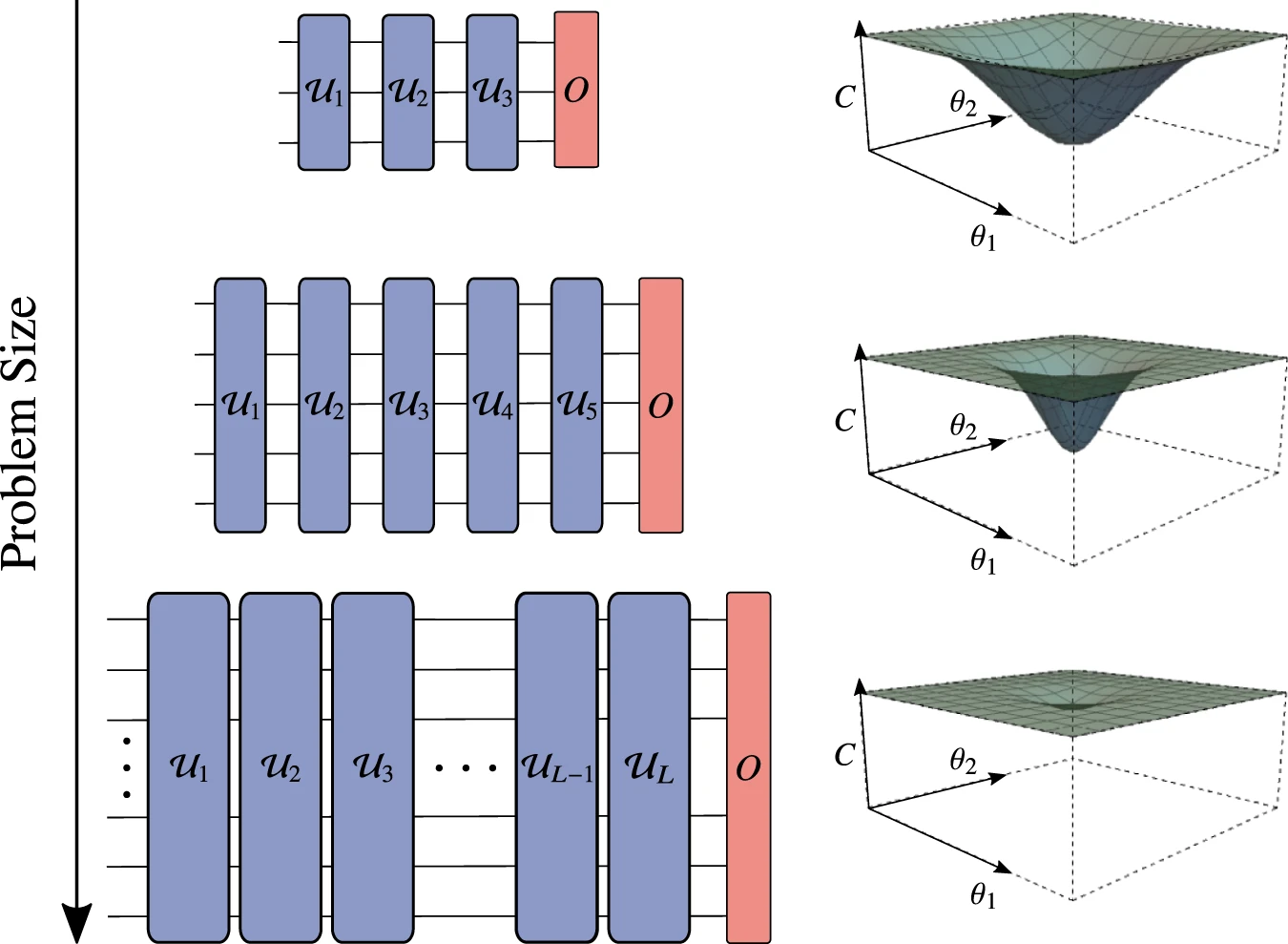
There are many solutions to this problem but the biggest comes from knowing a good initial Ansatz. If we choose an ansatz that is not on the plateau, then we are more likely to converge to at least a local minimum of the cost function. Another way of solving this comes from reducing the size of the problem. This is why many people are looking into algorithms that minimize the pauli weight and number of strings. There are best algorithms that can be implimented to do this, these are discussed in Jules Tilly.

The VQE Loop #

Now that our problem is set up, we need to talk about the illusive measurement question. Unfortunately, there are few good informative sources on this issue despite it being the most important part of the algorithm. How do we compute the expectation value on a quantum computer? We know that the only measurements we can make are those that ask the final state of the qbit. Fortunately, we can rotate this qbit in whatever maner we care for such that this question can be used to compute an expectation value. To outline this process again, we look at the [O’Malley] paper.

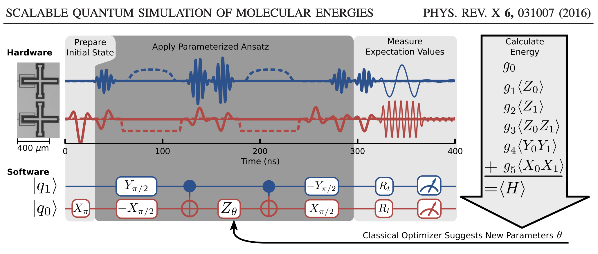
Circuit — **Fig.3.** Schematic of the VQE used in the O'Malley paper. They use an ansatz scheme called the unitary coupled cluster theroy.

In their algorithm, we see in Fig.3 that there are these \(R_t\) rotation matrices that encode the hamiltonian into the computational qbit basis in a way that a projective measurements can give information about these expectation values. We have allready expressed the Hamiltonian as a linear combination of these pauli strings, and we can compute the energy by the following

\[\begin{gather*} g_0\braket{I} \\ g_1\braket{Z_0} \\ g_2\braket{Z_1}\\ g_3\braket{Z_0Z_1} \\ g_4\braket{Y_0Y_1} \\ g_5\braket{X_0X_1}. \end{gather*}\]

If each of these expectation values we wanted where \(\braket{Z_1\otimes I_0}\) basis, then we could easily measure these expectation values by use of the the projective value measurement. But if instead we want to measure \(\braket{Y_1\otimes I_1}\), then we need to rotate the one qbit into the \(Y\) basis for measurement. This can be done by the following

\[ Y_1\otimes I = (HS^\dagger\otimes I)^\dagger(Z_1\otimes I)(HS^\dagger\otimes I) \]

Or for \(\braket{X_1\otimes I_1}\)

\[ X_1\otimes I = (H\otimes I)^\dagger(Z_1\otimes I)(H\otimes I) \]

Applying this, we get the make projective measurements for each of these pauli gates. After this algorithm runs, we get our six measurements, from these measurements, the classical computer determines an update for the parameters of the ansatz. In the case we are working with, this corresponds to updating \(\theta\) in the \(Z\) rotation gate.

The VQE is a way of ofloading the linear algebra from a classical computer to a quantum computer. Weather or not this offers any speedup will depend on the system of interest. In this example problem of \(H_2\), a classical computer can easily compute these things without any issues, and the Hamiltonian can be exactly diagonalized. If we where to try to run this on a quantum computer, the overhead of encoding the ansatz after every iteration loses much of the utility of the algorithm.

Outlook of VQE #

The VQE is currently one of the few algorithms that can make use of a quantum computer to solve for the ground state energy for quantum many-body systems. This being said, the implementation of this algorithm come with many issues; the choice between first and second quantization, the method of encoding the Hamiltonian, the choice in ansatz. Many of these issues have no definative best solution leading to a wide varity in the eficacy of these calculations. Even in the best case scenario for pre processing, there are still integrals that need to be computed for our system such as the \(g_i\) values in our example problem.

In class, Qiskit Nature was discussed where all the previously mentioned steps are glossed over as they have pre-built algorithms that generate the ansatz and circuit calling that the problem, then they use optimization algorithms to update their ansatz. However, they do all this in a very particular method that is not well described. For example, they restrict the user to use a second quantized form. At the same time, some argue that there can be problems where this may be problems where first quantized Hamiltonians provide computational benefits. In another example, they use Jordan-Wignar encoding while there are other encoding methods that can reduce the gate depth of the circuit.

Qiskit Nature’s VQE is reminiscent of Density Functional Theory platforms that are used by computational chemists to understand molecular electron structures. Some examples of these are StoBe, and DeMon 2k both of which provide easy-to-use software packages for doing DFT calculations. They have libraries of functionals and basis sets allowing for simple and fast computations using DFT treating it as some black box.

This comparison is perhaps the largest issue with Qiskit Nature and other similar packages. DFT has been shown to answer the same question as VQE for significantly more complex systems. For example, I have used it to compute the absorbtion sepctra for Zinc Phthalocyanine, an organic molecule with 32 carbon atoms to good qualetative agreement with experiments. This is something outside of the scope of the VQE in it’s entirety as the VQE only works for the ground state energy and has only been shown to work for small molecules per p. Lour.

**Fig.5.** An example calculation for ZnPc using a transition potential DFT scheme on StoBe.

Now, sure as the our quantum systems get larger VQU will be able to handle more complex Hamiltonians, but we will also have acess to better algorithms. An example of this is the quantum phase approximation algorithm that could give eigenvalues from an approximated ground or excited eigenstate. This algorithm is beyond the scope of NISQ devices but as quantum computation scales, it will become more fisable and the benifits of the VQE will begin to die out. An outline of this algorithm is also given by Jules Tilly.

As we mentioned before, there are three main problems that need to be answered before the algorithm can run. These being encoding of the Hamiltonian, grouping operations, and chosing an ansatz. Solutions to these problems can have applications in other fields in physics or data science. For example the barren plateau problem can be common across any large parameter space depending on the system. So, any improvements in these areas of the eigensolver can be applied to these similar problems. While within the field of qunatum information, these problems are similar to many other quantum optimization problems, as they work in similar ways. So, despite the gloomy outlook on this particular algorithm research in it is not entirely a lost cause.