import sys
print(sys.executable)
/home/docs/checkouts/readthedocs.org/user_builds/physics-555-quantum-technologies/conda/latest/bin/python3
%matplotlib inline
import numpy as np, matplotlib.pyplot as plt
import mmf_setup;mmf_setup.nbinit()
This cell adds /home/docs/checkouts/readthedocs.org/user_builds/physics-555-quantum-technologies/checkouts/latest/src to your path, and contains some definitions for equations and some CSS for styling the notebook. If things look a bit strange, please try the following:
- Choose "Trust Notebook" from the "File" menu.
- Re-execute this cell.
- Reload the notebook.
Designing Potentials#
Consider a single particle in a 1D potential:
Can we design the potential \(V(x)\) to obtain a desired spectrum?
Example Problem: Spectral Gap#
For example, supposed we want to consider localized solutions, so we consider solutions embedded in an infinite square well \(V(x) = \infty\) if \(x<0\) or \(L < x\). Can we design a potential \(V(x)\) with two low-energy states \(E_0 = 0\) and \(E_1 = E\) but a spectral gap \(\Delta\) so that all higher energy states \(E_{n>1} > E + \Delta\) for arbitrary large \(\Delta\)?
Let’s start with some fundamental properties of the 1D Schrödinger equation. We know that we can take the eigenstates \(\psi_n(x) = \braket{x|\psi} = \psi_n^*(x)\) to be real, and that \(\psi_{n}(x)\) has \(n\) nodes where \(\psi_n(x) = 0\). Thus, we can construct the potential from the ground state wavefunction and energy:
Infinite Square Well#
We start with \(V(x) = 0\). This has the well known solution
Show code cell source
import scipy.linalg
sp = scipy
# Check orthonormality of solution.
hbar = m = L = 1.2
Nx = 200
NE = 10
# This is a nice numerical trick: we choose Nx points between 0 and L
# such that they are separated by lattice space dx, but start and end
# dx/2 from the endpoints. Thus (Nx-1)*dx + 2*dx/2 = Nx*dx = L.
# Choosing the endpoints to be dx/2 away from 0 and L improves the accuracy
# of numerical integration.
dx = L / Nx
x = dx/2 + np.arange(Nx)*dx
n = np.arange(NE)
k_n = np.pi*(1+n)[np.newaxis, :]/L
psi_n = np.sqrt(2/L) * np.sin(k_n*x[:, np.newaxis])
# Check orthonormality
assert np.allclose(psi_n.T.conj() @ psi_n * dx, np.eye(NE))
#plt.plot(x, psi_n)
def get_H_basis(L=1.0, Nx=200, hbar2_m=hbar**2/m):
dx = L / Nx
x = dx/2 + np.arange(Nx)*dx
n = np.arange(Nx)
k_n = np.pi*(1+n)/L
Es = (hbar2_m * k_n**2/2)
psis = np.sqrt(2/L) * np.sin(k_n[np.newaxis, :]*x[:, np.newaxis])
# Not sure why we need this, but it gives an exactly orthonormal basis.
psis[:, -1] /= np.sqrt(2)
return x, Es, psis * np.sqrt(dx)
# 3000 -> 2292
# 2000 -> 1515
# 1000 -> 742
# 100 -> 57
# 50 -> 23
# 20 -> 4
# 10 -> 2
# Ne = 7*Nx/9 - 30
Nx = 200
Ne = int(Nx*0.77 - 20) # Emperical number energy states accurate to eps...
x, Es, psis = get_H_basis(Nx=Nx)
assert np.allclose(psis.T.conj() @ psis, np.eye(len(x)))
# Test with half HO
# Set length so ground state fits to machine eps
a = L / np.sqrt(-np.log(np.finfo(float).eps))
# Now divide by a factor so that the Ne state fits... explain!
# Tested emperically.
a /= np.sqrt(Nx/8)
w = hbar/m/a**2
Vx = m * (w*x)**2/2
H = np.diag(Es) + (psis.T * Vx) @ psis
E_HO = hbar*w*(2*np.arange(len(Es)) + 1 + 0.5)
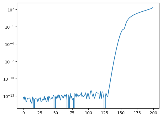
plt.semilogy(abs((sp.linalg.eigvalsh(H) - E_HO) / hbar / w))
assert np.allclose(sp.linalg.eigvalsh(H)[:Ne], E_HO[:Ne])
#display(E_HO / hbar / w)
#display(sp.linalg.eigvalsh(H) / hbar / w)
def get_spectrum(V, Nx=200):
H = np.diag(Es) + (psis.T * V(x)) @ psis
return sp.linalg.eigvalsh(H)
from scipy.optimize import minimize
Nx = 100
x, Es, psis = get_H_basis(Nx=Nx)

Np = 10
rng = np.random.default_rng(seed=1)

bounds = np.ones((2, Np, 2))
bounds[0, :, 0] = -20.0
bounds[0, :, 1] = 20.0
bounds[1, :, 0] = 0.0
bounds[1, :, 1] = 10.0
bounds = bounds.reshape((2*Np, 2))

def pack(x, v):
    y = np.concatenate([v, dx])
    return y

def unpack(y):
    # len(y) = 2*Np
    Np = len(y) // 2
    v, dx = y[:Np], y[Np:]
    _x = np.concatenate([[0], np.cumsum(dx)]) * L / np.sum(dx)
    _v = np.concatenate([[0], v])
    return _x, _v

def gap(y):
    _x, _v = unpack(y)
    Vx = np.interp(x, _x, _v)
    H = np.diag(Es) + (psis.T * Vx) @ psis
    _Es = sp.linalg.eigvalsh(H)[:3]
    dEs = np.diff(_Es)
    gap = dEs[1]/dEs[0]
    print(gap, _Es)
    return -gap

y0 = rng.random(size=(2, Np))
y0[0] -= 0.5
y0[0] *= bounds[0,1]
y0[1] *= bounds[-1,1]
y0 = y0.ravel()

res = minimize(gap, x0=y0, bounds=bounds)
Vx = np.interp(x, *unpack(res.x))
H = np.diag(Es) + (psis.T * Vx) @ psis
_Es, _Vs = sp.linalg.eigh(H)
Psis = psis @ _Vs[:, :3]
plt.close('all')
plt.plot(x, Vx, x, Psis*abs(Vx.max()) + _Es[None, :3])
Transfer Matrix#
Now consider the potential to be a series of \(S\) steps of height \(V_s\) over \(S\) regular intervals:
This problem can be solved using a transfer-matrix approach. If the potential \(V(x) = V_s\) is constant for \(0<x<a\), then the solution with energy \(E_s\) must satisfy:
Since the Schrödinger equation is second order, to “propagate” the wavefunction \(\psi(x)\) from \(x=0\) to \(x=a\), we need two initial conditions at \(x=0\), which we package as an array. For example:
Using the exact solution, and a little symbolic manipulation, we can write:
The second (equivalent) form is useful if \(E_s < V_s\):
Show code cell content
# Some code to test this formula.

import sympy
sympy.var('A, B, k, a, x, x_0, psi0, psia, dpsia')
dpsi0 = sympy.var(r"\psi'_0")

def psi(x):
    return A*sympy.exp(sympy.I*k*x) + B*sympy.exp(-sympy.I*k*x)

_dpsi = psi(x).diff(x)
dpsi = lambda _x: _dpsi.subs(x, _x)

eqs = [psi(x_0)-psi0, psi(x_0+a)-psia, dpsi(x_0)-dpsi0, dpsi(x_0+a)-dpsia]
res = sympy.solve(eqs, [A, B, psia, dpsia])
psia, dpsia = res[psia], res[dpsia]
T = sympy.simplify(
  sympy.Matrix([
    [psia.coeff(psi0), psia.coeff(dpsi0)],
    [dpsia.coeff(psi0), dpsia.coeff(dpsi0)]]))
display(T)
Since the wavefunction and derivative must be continuous across different regions, we can transfer the wavefunction over a series of intervals by simply multiplying the matrices \(\mat{T}=\mat{T_{S-1}}\cdots\mat{T_2}\mat{T_1}\mat{T_0}\).
Delta Functions#
This transfer matrix approach can also be used with Dirac delta-function potentials \(V(x) = α δ(x)\). Across a delta-function, the wavefunction remains continuous, but the derivative can change, resulting in a kink. This can be found by integrating the Schrödinger equation across the delta-function, which we take at \(x=0\) for simplicity
Hence, the transfer matrix across a delta-function is:
Note
The more common approach for the transfer-matrix is to express
Matching the boundary conditions at \(x=a\) between intervals \(s\) and \(s+1\) gives
Solving for \(\vec{\phi}_{s+1}\) we have (see [Walker and Gathright, 1992]: James S. Walker was a professor in the WSU Physics department):
Then
so we can write:
Thus, we can express \(\psi(a)\) and \(\psi'(a)\) in terms of \(\psi(0)\) and \(\psi'(0)\):
If \(V(x) = V_s\) is constant for \(x_0 < x < x+a\) and we know \(\psi_s(x_0)\) and \(\psi_s'(x_0)\), then we can integrate the Schrödinger equation to obtain \(\psi_s(x)\) throughout the interval.
To see how this works, consider the interval from \(x_0 = 0\) to \(x=0\). The solution must have the form:
Let \(\psi(x)\)
Write the wavefunction corresponding to energy \(E=E_n\) in each interval as:
If the wavefunction is $
Delta-Functions#
Here is one solution – a symmetric infinite square well with three delta function potentials,
This is easily solved with our transfer matrix approach:
import numpy as np
from ipywidgets import interact

a = hbar = m = 1.0
Nx = 256

E4 = hbar**2 * np.pi**2 / 2 / m / a**2

@interact(E=(0, 2*E4, 0.01))
def get_psi(E=E4, alpha=10.0, beta=20.0):
    k = np.sqrt(2*m*abs(E))/hbar
    if E < 0:
        def Ts(x):
            c, s = np.cosh(k*x), np.sinh(k*x)
            return np.array(
                [[c, s/k],
                 [k*s, c]])
    else:
        def Ts(x):
            c, s = np.cos(k*x), np.sin(k*x)
            return np.array(
                [[c, s/k],
                 [-k*s, c]])
    Ta = np.array(
        [[1, 0],
         [2*m*alpha/hbar**2, 1]])
    Tb = np.array(
        [[1, 0],
         [2*m*beta/hbar**2, 1]])

    Psis = [[0, 1]]
    Psis.append(Ta @ Ts(a) @ Psis[-1])
    Psis.append(Tb @ Ts(a) @ Psis[-1])
    Psis.append(Ta @ Ts(a) @ Psis[-1])
    Psis.append(Ts(a) @ Psis[-1])
    x = np.linspace(0, a, Nx//4)[:-1]
    psi = np.concatenate([np.einsum('abx,b->ax', Ts(x), _Psi)[0]
                          for _Psi in Psis[:-1]])
    x = np.concatenate([x + _n*a for _n in range(len(Psis)-1)]) - 2*a
    psi = np.concatenate([psi, [(Ts(a) @ Psis[-2])[0]]])
    x = np.concatenate([x, [2*a]])

    fig, ax = plt.subplots()
    ax.plot(x, psi)
    ax.axhline([0], ls='--', c='k')
---------------------------------------------------------------------------
ModuleNotFoundError                       Traceback (most recent call last)
Cell In[5], line 2
      1 import numpy as np
----> 2 from ipywidgets import interact
      4 a = hbar = m = 1.0
      5 Nx = 256

ModuleNotFoundError: No module named 'ipywidgets'
def get_Ts(E, x=a):
    k = np.sqrt(2*m*abs(E))/hbar
    if E == 0:
        Ts = np.array(
            [[1, x],
             [0, 1]])
    elif E < 0:
        c, s = np.cosh(k*x), np.sinh(k*x)
        Ts = np.array(
            [[c, s/k],
             [k*s, c]])
    else:
        c, s = np.cos(k*x), np.sin(k*x)
        Ts = np.array(
            [[c, s/k],
             [-k*s, c]])
    return Ts

@np.vectorize
def f(E=1.0, alpha=1.0, beta=2.0):
    Ts = get_Ts(E=E, x=a)
    Ta = np.array(
        [[1, 0],
         [2*m*alpha/hbar**2, 1]])
    Tb = np.array(
        [[1, 0],
         [2*m*beta/hbar**2, 1]])

    Psi = Ts @ Ta @ Ts @ Tb @ Ts @ Ta @ Ts @ [0, 1]
    return Psi[0]

@interact
def go(alpha=10.0, beta=10.0):
    Es = np.linspace(0, 10, 256)
    fig, ax = plt.subplots()
    ax.plot(Es, f(Es, alpha=alpha, beta=beta))
    ax.axhline([0], ls='--', c='k')
    ax.axvline([E4])
    ax.set(ylim=(-1, 1))
---------------------------------------------------------------------------
NameError                                 Traceback (most recent call last)
Cell In[6], line 32
     29     Psi = Ts @ Ta @ Ts @ Tb @ Ts @ Ta @ Ts @ [0, 1]
     30     return Psi[0]
---> 32 @interact
     33 def go(alpha=10.0, beta=10.0):
     34     Es = np.linspace(0, 10, 256)
     35     fig, ax = plt.subplots()

NameError: name 'interact' is not defined
import sympy
sympy.var('a, alpha, beta, x, hbar, m, E')
#sympy.var('E', positive=True)
#a = hbar = m = 1
hbar2_m = hbar**2/m
a = hbar2_m = 1

def get_Ts(E=E, a=a, V=0):
    k = sympy.sqrt(2*(V-E)/hbar2_m)
    c, s = sympy.cos(k*a), sympy.sin(k*a)
    return sympy.Matrix([
        [c, s/k],
        [-k*s, c]])

def get_Td(a):
    return sympy.Matrix([
        [1, 0],
        [2*a/hbar2_m, 1]])

Ta, Tb, Ts = get_Td(alpha), get_Td(beta), get_Ts(E, a=a)
psi_R = (Ts * Ta * Ts * Tb * Ts * Ta * Ts * sympy.Matrix([[0],[1]]))[0,0]
res = sympy.simplify(psi_R)
res