Weak Measurements#

The generalized Measurement formalism allows for a simplified discussion of weak measurements. The idea is to introduce a set of Kraus operators \(\{\mat{M}_{m}\}\) that are in some sense close to the identity \(\mat{M}_{m} \approx a\mat{1}\) (with a proportionality factor) such that the measurements do not completely collapse the state. Here we consider a simple example and explore how weak measurements can be used to advantage when interrogating quantum systems.

Single Qubit Example#

Consider the following weak measurements of \(\mat{Z}\):

\[\begin{gather*} M_\alpha = \{\mat{M}_{+1}, \mat{M}_{-1}\},\\ \mat{M}_{+1} = \frac{1}{\sqrt{1+\alpha^2}}\begin{pmatrix} 1\\ & \alpha \end{pmatrix}, \qquad \mat{M}_{-1} = \frac{1}{\sqrt{1+\alpha^2}}\begin{pmatrix} \alpha\\ & 1 \end{pmatrix},\\ \mat{E}_{+1} = \frac{1}{1+\alpha^2}\begin{pmatrix} 1\\ & \alpha^2 \end{pmatrix}, \qquad \mat{E}_{-1} = \frac{1}{1+\alpha^2}\begin{pmatrix} \alpha^2\\ & 1 \end{pmatrix},\\ \mat{E}_{\pm 1} = \tfrac{1}{2}(\mat{1} \pm \epsilon\mat{Z}), \qquad \epsilon = \frac{1 - \alpha^2}{1+\alpha^2}, \qquad \alpha^2 = \frac{1 - \epsilon}{1+\epsilon}, \end{gather*}\]

where we call \(\epsilon\) the weakness parameter.

Do it! Implement these using projective measurements.

These can be implemented as strong measurements of the following operators, which make use of a single qubit ancillae. First define a unitary operator \(\mat{U}\) that behaves as follows

\[\begin{gather*} \mat{U}\ket{\psi}\ket{0} = \sum_{m=\pm} \mat{M}_{m}\ket{\psi}\ket{m} \tag{2.122}. \end{gather*}\]

If \(\epsilon = 1\) (\(\alpha = 0\)), these correspond to the standard von Neumann measurement of \(\op{Z}\), but as \(\epsilon \rightarrow 0\) (\(\alpha \rightarrow 1\)), they provide less and less information about the state, but also cause less of a collapse. In the extreme limit \(\epsilon = 0\), we have \(\mat{M}_{+1} = \mat{M}_{-1} = \mat{1}/\sqrt{2}\), and the measurement leaves the state undisturbed, while providing absolutely no information.

To visualize what these measurements tell us, consider an initial state

\[\begin{gather*} \ket{\theta} = \cos\tfrac{\theta}{2}\ket{0} + \sin\tfrac{\theta}{2}\ket{1} \end{gather*}\]

with \(\theta \in [0, \pi]\). Measuring this state gives \(m \in \{+1, -1\}\) with probabilities

\[\begin{gather*} p_\epsilon(+1|\theta) = \frac{\cos^2\tfrac{\theta}{2} + \alpha^2\sin^2\tfrac{\theta}{2}}{1+\alpha^2} = \frac{1}{2}\left(1 + \epsilon\cos\theta\right),\\ p_\epsilon(-1|\theta) = \frac{\alpha^2\cos^2\tfrac{\theta}{2} + \sin^2\tfrac{\theta}{2}}{1+\alpha^2} = \frac{1}{2}\left(1 - \epsilon\cos\theta\right). \end{gather*}\]

More succinctly:

\[\begin{gather*} p_\epsilon(m|\theta) = \tfrac{1}{2}(1 + m\,\epsilon\cos\theta) \end{gather*}\]

What about the action of the measurement on the state? According to the postulate of generalized measurements, \(\ket{\psi} \rightarrow \mat{M}_{m}\ket{\psi}/\sqrt{p_m}\). Thus:

\[\begin{gather*} \mat{M}_{+1}\ket{\theta} \propto \begin{pmatrix} \cos\tfrac{\theta}{2}\\ \alpha\sin\tfrac{\theta}{2} \end{pmatrix}, \qquad \mat{M}_{-1}\ket{\theta} \propto \begin{pmatrix} \alpha\cos\tfrac{\theta}{2}\\ \sin\tfrac{\theta}{2} \end{pmatrix}. \end{gather*}\]

Since these \(\mat{M}_{\pm 1}\) commute (they are both diagonal), we can succinctly describe a series of \(n_{+}\) measurements with value \(m=+1\) and \(n_{-}\) measurements with value \(m=-1\):

\[\begin{gather*} \mat{M}_{+1}^{n_{+}}\mat{M}_{-1}^{n_{-}}\ket{\theta} \propto \begin{pmatrix} \alpha^{n_-}\cos\tfrac{\theta_n}{2}\\ \alpha^{n_+}\sin\tfrac{\theta_n}{2} \end{pmatrix} \propto \begin{pmatrix} \cos\tfrac{\theta_{n_+-n_-}}{2}\\ \sin\tfrac{\theta_{n_+-n_-}}{2} \end{pmatrix} = \ket{\theta_{n_{+}-n_{-}}}, \\ \tan\tfrac{\theta_{n_{+}-n_{-}}}{2} = \frac{\alpha^{n_{+}}}{\alpha^{n_{-}}}\tan\tfrac{\theta}{2} = \alpha^{n_{+}-n_{-}}\tan\tfrac{\theta}{2}. \end{gather*}\]

Generalizing slightly and using rotational invariance, we will also consider measurements at an angle \(\vartheta\) – i.e. \(\vartheta=\pi/2\) corresponds to a weak measurement of \(\mat{X}\) – with probabilities:

\[\begin{gather*} p_{\epsilon,\vartheta}(m|\theta) = p_{\epsilon}(m|\theta-\vartheta) = \frac{1}{2}\left( 1 + m,\epsilon\cos(\theta-\vartheta) \right),\\ \mat{M}_{m}(\vartheta)\ket{\theta} \propto \ket{\theta_{m}}, \qquad \tan\tfrac{\theta_{m}-\vartheta}{2} = \alpha^{m}\tan\tfrac{\theta-\vartheta}{2}. \end{gather*}\]

Thus, the weak measurement has the effect of marching the state towards the measurement eigenstates, but with decreasing step size.

Random Walk on Bloch Sphere#

To make this behavior a little more explicit, it is useful to introduce some new variables:

\[\begin{gather*} x = -\ln \tan\tfrac{\theta}{2}, \qquad \delta = -\ln \alpha = \tanh^{-1}\epsilon. \end{gather*}\]

In terms of these variables, the evolution under these weak measurements is exactly that of a random walk with step size \(\delta\)

\[\begin{gather*} x \mapsto x + m\delta \end{gather*}\]

where \(m = \pm 1\) is a random variable with distribution that depends on \(x\):

\[\begin{gather*} p_\delta(m|x) = \tfrac{1}{2}(1 + m\,\epsilon\,\tanh x) = \tfrac{1}{2}(1 + m\tanh\delta\,\tanh x). \end{gather*}\]

Information and Bayes’ Theorem#

We now ask the question: What can we learn about a state by performing measurements. To make this definite, suppose we are given a quantum state \(\ket{\theta}\) known to lie in the \(x-z\) plane, but with some prior knowledge coded in the prior distribution \(p(\theta)\).

After making a measurement with outcome \(m\), we can characterize what we have learned by using Bayes’ theorem to get the posterior distribution

\[\begin{gather*} p_\epsilon(\theta|m) \propto p_\epsilon(m|\theta)p(\theta), \end{gather*}\]

where \(p_\epsilon(m|\theta)\) is the likelihood of measuring \(m\) if the state is \(\ket{\theta}\).

Now consider a sequence of measurements giving results \(\vect{m} = [m_1, m_2, \cdots]\). Our posterior changes as:

\[\begin{align*} p_{\epsilon;\vartheta_1}(\theta|m_1) &\propto p_{\epsilon,\vartheta_1}(m_1|\theta)p(\theta),\\ p_{\epsilon;\vartheta_1,\vartheta_2}(\theta|m_1,m_2) &\propto p_{\epsilon,\vartheta_2}(m_2|\theta_1)p_{\epsilon;\vartheta_1}(\theta|m_1),\\ p_{\epsilon;\vartheta_1,\vartheta_2,\vartheta_3}(\theta|m_1,m_2,m_3) &\propto p_{\epsilon,\vartheta_3}(m_3|\theta_2)p_{\epsilon;\vartheta_1,\vartheta_2}(\theta|m_1,m_2),\\ &\;\;\vdots\\ p_{\epsilon;\vec{\vartheta}}(\theta|\vect{m}) &\propto p(\theta)\prod_{i=1}^{n} p_{\epsilon,\vartheta_i}(m_i|\theta_{i-1}). \end{align*}\]

where \(\theta_n\) characterizes the evolution of the state.

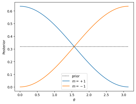
As a specific example, first consider a strong measurement along \(\vartheta = 0\) yielding the result \(m=\pm 1\) with a uniform prior \(p(\theta)=1/\pi\). The normalized posteriors are:

\[\begin{gather*} p(\theta|m) = \frac{1 + m\cos(\theta)}{\pi}. \end{gather*}\]

../_images/b851ea0e4cde90f3d4c145281fcbc31ecba57bf64c58dc7d8d16f01f51d06ec6.png

Now, suppose we start with state \(\ket{\theta=0} = \ket{0}\) (but we do not know this… we still assume our prior is uninformed \(p(\theta) = 1/\pi\)). In this particular case, a sequence of measurements will always give \(m = +1\). We must, however, still evolve \(\theta_n\) in our likelihood function: \(\tan\tfrac{\theta_{n}}{2} = \alpha^{n}\tan\tfrac{\theta}{2}\).

Here are the results of performing a series of weak measurements in this case:

---------------------------------------------------------------------------
NameError                                 Traceback (most recent call last)
Cell In[5], line 48
     46 ax.plot(thetas, p0, '-k', label=r"$\epsilon=1$")
     47 p1 = posterior(ps[0], epsilon=1, theta=thetas, m=1)
---> 48 ax.plot(thetas, p1, '-k', label=fr"$\epsilon=1$, $H(p‖p_0)={H(p1, p0):.2f}$")
     49 ax.set(xlabel=fr"$\theta$", 
     50       ylabel=r"Posterior $p(\theta)$ after $n$ measurements",
     51       title=fr"$\epsilon={epsilon}$")
     52 ax.legend()

NameError: name 'H' is not defined

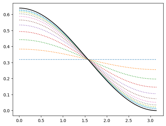
../_images/9b63f219d34c078c89be7bd53ddd79ed4cc968e8c08f99081fea0a9f124a0279.png

We see that a sequence of weak measurements approaches the result of a single strong measurement (or a sequence of strong measurements since a sequence is equivalent to a single strong measurement). Thus, in this case, weak measurements provide no advantage over a strong measurement.

Information Theory I#

How might we characterize: “how much we learn” by making these measurements? One way is to use the von Neumann entropy of the distribution:

\[\begin{gather*} \end{gather*}\]

Incomplete…#

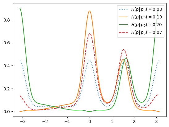
Where might we gain an advantage? Perhaps if the prior is not uniform: weak measurements would allow one to check several different directions, whereas a strong measurement would collapse the system. To consider this, we use the same system where the actual underlying state is \(\ket{0}\), but now suppose we have two independent particles that we can measure. To be precise:

We have an underlying system of particles in the state \(\ket{0}\), but with a flat prior.
We consider making different measurements with the detector at angle \(\vartheta_{n}\), recording the results as \(m_{n}\) or \(s_n = 1-2m_n\). Using rotational invariance, we can deduce that the likelihood of measuring \(s\) with the detector at angle \(\vartheta\) and the state at angle \(\theta\) is:

\[\begin{gather*} p_{\alpha,\vartheta}(s|\theta) = p_{\alpha}(s|\theta-\vartheta) = \frac{1}{2}\left( 1 + s\frac{1-\alpha^2}{1+\alpha^2}\cos(\theta-\vartheta) \right) \end{gather*}\]

The posterior after making the \(n\in\{1, 2, \cdots\}\) strong measurements with results \(\vect{s} = (s_1, s_2, \dots, s_n)\) is:

\[\begin{gather*} p(\theta|\vect{s}) \propto \prod_{n}p_{\vartheta_n}(s_n|\theta)p(\theta). \end{gather*}\]

Consider now a measurement of the second particle in the direction of \(\theta^{m}_2\). The posterior now is:

Show code cell source Hide code cell source

from scipy.special import xlogy

_TINY = np.finfo(float).tiny

def likelihood(theta, vartheta, epsilon, m):
    """Return the likelihood of measuring m, given a state |theta>"""
    if m == -1:
        epsilon *= -1
    return (1 + epsilon*np.cos(theta-vartheta))/2

def measure(theta, vartheta, epsilon, m):
    """Perform the specified measurement and return the new theta."""
    alpha = np.sqrt((1-epsilon)/(1+epsilon))
    return vartheta + 2*np.arctan(alpha ** m * np.tan((theta-vartheta)/2))

def get_posterior(theta, epsilon, ms, varthetas):
    thetas = theta
    post = 0*thetas + 1/np.pi
    for m, vartheta in zip(ms, varthetas):
        kw = dict(theta=thetas, vartheta=vartheta, epsilon=epsilon, m=m)
        post = post * likelihood(**kw)
        thetas = measure(**kw)
    return post

rng = np.random.default_rng(seed=4)

def doit(theta, epsilon, N=10):
    """Do a series of measurements."""
    ms = []
    varthetas = []
    vartheta = 0
    for n in range(N):
        p0 = likelihood(theta, vartheta=vartheta, epsilon=epsilon, m=1)
        m = 1 if rng.random() < p0 else -1
        varthetas.append(vartheta)
        ms.append(m)
        if m == -1:
            vartheta = np.pi/2 - vartheta
    return ms, varthetas
    
def H(p, p0, theta=thetas):
    """Return the relative entropy H(p‖p_0)."""
    return np.trapz(xlogy(p, p/(p0+_TINY)), theta)
    
N = 200
thetas = np.linspace(-np.pi, np.pi, 2*N+1)[1:-1:2]

# Uninformed prior for comparison.
p0 = 0*thetas + 1/2/np.pi
ps = [p0]
theta = thetas

epsilon = 0.2
alpha = np.sqrt((1-epsilon)/(1+epsilon))

P0 = get_posterior(thetas, epsilon=1, ms=[1], varthetas=[0])
P1 = get_posterior(thetas, epsilon=1, ms=[-1], varthetas=[0])

ms, varthetas = doit(theta=np.pi/2, epsilon=epsilon, N=100)
P = get_posterior(thetas, epsilon=epsilon, ms=ms, varthetas=varthetas)

sigma = 1/4
p0 = (np.exp(-thetas**2/2/sigma**2) 
      + np.exp(-(thetas-np.pi/2)**2/2/sigma**2)
      + np.exp(-(thetas-np.pi)**2/2/sigma**2)
      + np.exp(-(thetas+np.pi)**2/2/sigma**2)
     ) + 0.1
p0 /= np.trapz(p0, thetas)

P0 *= p0
P1 *= p0
P *= p0
P0 /= np.trapz(P0, thetas)
P1 /= np.trapz(P1, thetas)
P /= np.trapz(P, thetas)
plt.plot(thetas, p0, ':', label=f"$H(p‖p_0)={H(p0, p0):.2f}$")
plt.plot(thetas, P0, label=f"$H(p‖p_0)={H(P0, p0):.2f}$")
plt.plot(thetas, P1, label=f"$H(p‖p_0)={H(P1, p0):.2f}$")
plt.plot(thetas, P, '--', label=f"$H(p‖p_0)={H(P, p0):.2f}$")
plt.legend();

/tmp/ipykernel_4850/984981411.py:14: RuntimeWarning: divide by zero encountered in scalar power
  return vartheta + 2*np.arctan(alpha ** m * np.tan((theta-vartheta)/2))

../_images/6b3315bd90c37c5e298e50fd3e30aa36e5f83f353655c5b3f2cb24759b6072a4.png

vartheta = np.pi/2
theta = np.pi/3
for n in range(10):
    print(theta)
    theta = measure(theta, vartheta=vartheta, epsilon=epsilon, m=1)

0471975511965976
140024432184815
2172596758834402
281132686307852
3337357304245163
3769350069520372
4123439785134186
4413302969180168
4650385386002653
484418626293319

'\nfor n in range(9):\n    ps.append(posterior(prior=ps[-1], epsilon=epsilon, theta=theta, m=0))\n    theta = 2 * np.arctan(alpha * np.tan(theta/2))\n\n\nfig, ax = plt.subplots()\nfor n, p in enumerate(ps):\n    ax.plot(thetas, p, \':\', label=f"$n={n}$, $H(p‖p_0)={H(p, p0):.2f}$")\n\np1 = posterior(ps[0], epsilon=1, theta=thetas, m=0)\nax.plot(thetas, p1, \'-k\', label=fr"$\\epsilon=1$, $H(p‖p_0)={H(p1, p0):.2f}$")\nax.set(xlabel=fr"$\theta$", \n      ylabel=r"Posterior $p(\theta)$ after $n$ measurements",\n      title=fr"$\\epsilon={epsilon}$")\nax.legend();\n'