JupyterBook Demonstration#

This document demonstrates some of the features provided by the documentation. It can serve as a starting point for your own documentation.

This documentation is formatted using an extension to Markdown called MyST which allows full interoperability with Sphinx, the system used to build the documentation. Here we demonstrate some features. For more details, please see:

Math#

You can use LaTeX math with [MathJaX]:

Example#

Here we implement a simple example of a pendulum of mass \(m\) hanging down distance \(r\) from a pivot point in a gravitational field \(g>0\) with coordinate \(\theta\) so that the mass is at \((x, z) = (r\sin\theta, -r\cos\theta)\) and \(\theta=0\) is the downward equilibrium position:

\[\begin{gather*} L(\theta, \dot{\theta}, t) = \frac{m}{2}r^2\dot{\theta}^2 + mgr\cos\theta\\ p_{\theta} = \pdiff{L}{\dot{\theta}} = mr^2 \dot{\theta}, \qquad \dot{\theta}(\theta, p_{\theta}, t) = \frac{p_{\theta}}{mr^2},\\ H(\theta, p_{\theta}) = p_{\theta}\dot{\theta} - L = \frac{p_{\theta}^2}{2mr^2} - mgr\cos\theta,\\ \vect{y} = \begin{pmatrix} \theta\\ p_{\theta} \end{pmatrix},\qquad \dot{\vect{y}} = \begin{pmatrix} 0 & 1\\ -1 & 0 \end{pmatrix} \cdot \begin{pmatrix} \pdiff{H}{\theta}\\ \pdiff{H}{p_{\theta}} \end{pmatrix} = \begin{pmatrix} p_{\theta}/mr^2\\ -mgr\sin\theta \end{pmatrix}. \end{gather*}\]

Note

On [CoCalc], only a subset of the math will render in the live Markdown editor. This uses KaTeX, which is much faster than [MathJaX], but more limited. The final documentation will use [MathJaX], and loads the macros defined in Docs/_static/math_defs.tex.

Jupyter Notebooks#

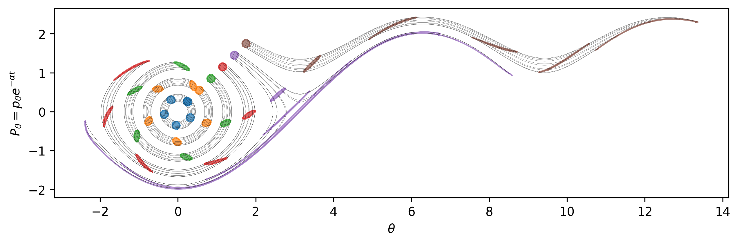
This document is actually a Jupyter notebook, synchronized with Jupytext. The top of the document contains information about the kernel that should be used etc. These are parsed using MyST-NB and the output of cells will be displayed. For example, here is a plot demonstrating Liouville’s Theorem.

Show code cell source Hide code cell source

plt.rcParams['figure.dpi'] = 300
from scipy.integrate import solve_ivp

alpha = 0.0
m = r = g = 1.0
w = g/r
T = 2*np.pi / w   # Period of small oscillations.


def f(t, y):
    # We will simultaneously evolve N points.
    N = len(y)//2
    theta, p_theta = np.reshape(y, (2, N))
    dy = np.array([p_theta/m/r**2*np.exp(-alpha*t),
                   -m*g*r*np.sin(theta)*np.exp(alpha*t)])
    return dy.ravel()


# Start with a circle of points in phase space centered here
def plot_set(y, dy=0.1, T=T, phase_space=True, N=10, Nt=5, c='C0', 
             Ncirc=1000, max_step=0.01, _alpha=0.7, 
             fig=None, ax=None):
    """Plot the phase flow of a circle centered about y0.
    
    Arguments
    ---------
    y : (theta0, ptheta_0)
        Center of initial circle.
    dy : float
        Radius of initial circle.
    T : float
        Time to evolve to.
    phase_space : bool
        If `True`, plot in phase space $(q, p)$, otherwise plot in
        the "physical" phase space $(q, P)$ where $P = pe^{-\alpha t}$.
    N : int
        Number of points to show on circle and along path.
    Nt : int
        Number of images along trajectory to show.
    c : color
        Color.
    alpha : float
        Transparency of regions.
    max_step : float
        Maximum spacing for times dt.
    Ncirc : int
        Minimum number of points in circle.
    """
    global alpha
    skip = int(np.ceil(Ncirc // N))
    N_ = N * skip
    th = np.linspace(0, 2*np.pi, N_ + 1)[:-1]
    z = dy * np.exp(1j*th) + np.asarray(y).view(dtype=complex)
    y0 = np.ravel([z.real, z.imag])

    skip_t = int(np.ceil(T / max_step / Nt))
    Nt_ = Nt * skip_t + 1
    t_eval = np.linspace(0, T, Nt_)
    res = solve_ivp(f, t_span=(0, T), y0=y0, t_eval=t_eval)
    assert Nt_ == len(res.t)
    thetas, p_thetas = res.y.reshape(2, N_, Nt_)
    ylabel = r"$p_{\theta}$"
    if phase_space:
        ylabel = r"$P_{\theta}=p_{\theta}e^{-\alpha t}$"
        p_thetas *= np.exp(-alpha * res.t)
    
    if ax is None:
        fig, ax = plt.subplots()

    ax.plot(thetas[::skip].T, p_thetas[::skip].T, "-k", lw=0.1)
    for n in range(Nt+1):
        tind = n*skip_t
        ax.plot(thetas[::skip, tind], p_thetas[::skip, tind], '.', ms=0.5, c=c)
        ax.fill(thetas[:, tind], p_thetas[:, tind], c=c, alpha=_alpha)
    ax.set(xlabel=r"$\theta$", ylabel=ylabel, aspect=1)
    return fig, ax


fig, ax = plt.subplots(figsize=(10,5))


for n, y in enumerate(np.linspace(0.25, 1.75, 6)):
    plot_set(y=(y, y), c=f"C{n}", ax=ax)

_images/4ac20bc863d91457424e28088db5f99acbbe9369fb475198c4b9d1f107f39fa6.png

The small colored circular region is evolved forward in time according to the Hamiltonian equations. The trajectories of 10 equally spaced points are shown at 6 different times equally spaced from \(t=0\) to \(T = 2\pi\sqrt{r/g}\), the period of oscillation for small amplitude modes. At small energies (blue circle), the period is almost independent of the amplitude, and the circle stays together. As the energy increases (orange, green, and red), the period starts to depend more sensitively on the amplitude, and the initial circular region starts to shear. The purple region divides the two qualitatively different regions of rotation and libration, and gets stretched as some points oscillate and others orbit. The areas remain constant, despite this stretching, as a demonstration of Liouville’s theorem.

Details

We start a code-block with:

```{code-cell}
:tags: [hide-input, full-width]
...
```

This indicates that it is a code cell, to be run with python 3, and has some tags to make the cell and output full width, but hiding the code. (There is a link to click to show the code.)

If you need more control, you can glue the output to a variable, then load it as a proper figure, insert it in a table, etc.

Manim#

Your project was generated from a template without Manim support. To use, please regenerate the project with use_manim = "yes". the