Bound States in the 1D Schrödinger Equation#

Here we consider the problem of finding the energies \(E\) of bound states in a 1D potential:

\[\begin{gather*} -\frac{\hbar^2}{2m}\psi''(x) + V(x)\psi(x) = E\psi(x). \end{gather*}\]

To simplify the problem, let assume that the potential is zero \(V(\abs{x}>R) = 0\) for \(x\) outside of some region \(-R < x < R\). This excludes some interesting examples, but simplifies our analysis considerably.

We will also assume that \(V(x)\) is sufficiently smooth so that numerical integration techniques will converge if we choose a sufficiently small step size. If you want to deal with \(\delta\)-functions, then you must replace these with something smooth like gaussians and then take the limit of zero width after the computation.

Question#

Given some attractive potential \(V(x)\) with compact support, how can we determine the bound state energies?

How can you quickly estimate the ground state energy \(E_0\)?
How can you quickly use numerical techniques to refine this?

Do It!

Stop here and this about this. Can you come up a simple problem of this type, that you can quickly solve? Start with something easy, but think about how you might generalize your methods if someone gives you a similar problem in the future.

Hints:

Shooting#

There are many numerical techniques capable of solving the Schrödinger equation, but shooting is one of the easiest. The idea is to start with a guess for the wavefunction \(\psi(x_i)\) and its derivative \(\psi'(x_i)\) at some point \(x_i\), and then integrate forward to another point \(x_f\) trying match an appropriate boundary condition. Most numerical techniques require the differential equation to be specified as a first-order equation \(\vect{y}'(x) = f(x, \vect{y})\), so we use a vector \(\vect{y} = (\psi, \psi')\)

\[\begin{gather*} \diff{}{x}\overbrace{ \begin{pmatrix} \psi(x)\\ \psi'(x) \end{pmatrix} }^{\vect{y}(x)} = \overbrace{ \begin{pmatrix} \psi'(x)\\ \frac{2m}{\hbar^2}\Bigl(V(x) - E\Bigr)\psi(x) \end{pmatrix} }^{f(x,\vect{y}(x))}. \end{gather*}\]

This is pretty easy to implement, either by hand using Euler’s method or (better) Leapfrog integration, or using an adaptive routine like SciPy’s solve_ivp. The remaining challenges are:

Choose an appropriate integration range \(x\in [x_i, x_f]\).
Choose an appropriate initial state \(\vect{y}(x_i) = [\psi(x_i), \psi'(x_i)]\).
Choose an appropriate boundary condition at \(x_f\) to “shoot for”.

Do It!

Try to answer find appropriate boundary conditions.

Hints:

A Simple Numerical Solution#

Important

Do not work through this section until you have thought carefully about the problem and how you might try to solve. Ideally, you should try to solve it yourself, but if you are not very comfortable coding, then come here after you have thought about the math.

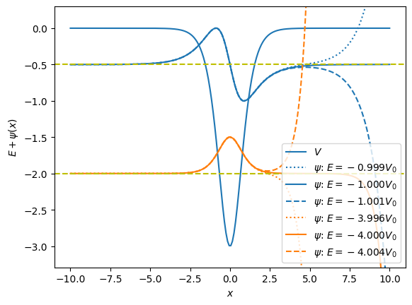
Let’s consider a the problem of a particle in the Pöschl-Teller potential:

\[\begin{gather*} V(x) = -\frac{n(n+1)\hbar^2}{2ma^2}\sech^2\frac{x}{a}, \end{gather*}\]

which has \(n\) bound states with energies

\[\begin{gather*} E_n = -\frac{n^2\hbar^2}{2ma^2}. \end{gather*}\]

We will use the Leapfrog integration scheme for a fixed step size.

# :tags: [hide-input, full-width]

hbar = m = a = 1.0
n = 2

V0 = hbar**2/2/m/a**2
ns = np.arange(1, n+1)
Es = -ns**2 * V0

def V(x, V0=V0, n=n):
    return -n*(n+1)*V0/np.cosh(np.asarray(x)/a)**2

dx = a/1000

xi = -10*a
xf = 10*a
Nsteps = int(np.ceil((xf-xi)/dx))

def shoot(E, xi=xi, xf=xf, Nsteps=Nsteps):
    """Return (xs, psis).
    
    Arguments
    ---------
    E : float
        Energy
    xi : float
        Initial point.
    xf : float
        Final point
    NSteps : int
        Number of steps.
    """
    dx = (xf-xi)/Nsteps

    # Initial ansatz... can be anything since the problem is linear
    psi = 0.1
    kappa = np.sqrt(-2*m*E)/hbar

    # Correct leapfrog initial guess using asymptotic form of wavefunction
    dpsi = kappa*psi*np.exp(kappa*dx/2)

    # Why does this work as well???
    #dpsi = 0

    x = xi
    xs = [xi]
    psis = [psi]
    for _n in range(Nsteps):
        ddpsi = 2*m*(V(x) - E)*psi/hbar**2
        dpsi += ddpsi * dx
        psi += dpsi * dx
        x += dx
        xs.append(x)
        psis.append(psi)

    xs, psis = map(np.asarray, (xs, psis))
    return xs, psis

fig, ax = plt.subplots()
xs = np.linspace(xi, xf, 200)
ax.plot(xs, V(xs), label="$V$")
V_min = np.min(V(xs))
for n, En in enumerate(Es):
    dE = 1.001
    xs, psis = shoot(E=En)
    max_psi = np.where(abs(V(xs)) > 0.1, abs(psis), 0).max()
    for E, ls in [(En/dE, ':'), (En, '-'),  (En*dE, '--')]:
        xs, psis = shoot(E=E)
        ax.plot(xs, E + psis*V0/max_psi, c=f"C{n}", ls =ls, 
                label=fr"$\psi$: $E={E/V0:.3f}V_0$")
    plt.axhline(En, ls='--', c='y')
    
ax.legend()
ax.set(xlabel="$x$", ylabel=r"$E + \psi(x)$", ylim=(1.1*V_min, 0.1*abs(V_min)));

../_images/dc73a790e9a2aad078162a2e81a0ec33c7439a8510cf232c8df8ced9d0d81051.png

To Ponder#

Notice that unless we tune the energy precisely, it diverges exponentially. Why?

Bound States in the 1D Schrödinger Equation

Contents

Bound States in the 1D Schrödinger Equation#

Question#

Shooting#

A Simple Numerical Solution#

To Ponder#