import sys
print(sys.executable)

/home/docs/checkouts/readthedocs.org/user_builds/physics-555-quantum-technologies/conda/latest/bin/python3

import mmf_setup;mmf_setup.nbinit()
import logging;logging.getLogger('matplotlib').setLevel(logging.CRITICAL)
%matplotlib inline
import numpy as np, matplotlib.pyplot as plt

$\newcommand{\vect}[1]{\mathbf{#1}} \newcommand{\uvect}[1]{\hat{#1}} \newcommand{\abs}[1]{\lvert#1\rvert} \newcommand{\norm}[1]{\lVert#1\rVert} \newcommand{\I}{\mathrm{i}} \newcommand{\ket}[1]{\left|#1\right\rangle} \newcommand{\bra}[1]{\left\langle#1\right|} \newcommand{\braket}[1]{\langle#1\rangle} \newcommand{\Braket}[1]{\left\langle#1\right\rangle} \newcommand{\op}[1]{\mathbf{#1}} \newcommand{\mat}[1]{\mathbf{#1}} \newcommand{\d}{\mathrm{d}} \newcommand{\D}[1]{\mathcal{D}[#1]\;} \newcommand{\pdiff}[3][]{\frac{\partial^{#1} #2}{\partial {#3}^{#1}}} \newcommand{\diff}[3][]{\frac{\d^{#1} #2}{\d {#3}^{#1}}} \newcommand{\ddiff}[3][]{\frac{\delta^{#1} #2}{\delta {#3}^{#1}}} \newcommand{\floor}[1]{\left\lfloor#1\right\rfloor} \newcommand{\ceil}[1]{\left\lceil#1\right\rceil} % The following allows KaTeX to render these for significantly improved % performance on CoCalc. \newcommand{\DeclareMathOperator}[2]{\newcommand{#1}{#2}} \DeclareMathOperator{\Tr}{Tr} \DeclareMathOperator{\erf}{erf} \DeclareMathOperator{\erfi}{erfi} \DeclareMathOperator{\sech}{sech} \DeclareMathOperator{\sn}{sn} \DeclareMathOperator{\cn}{cn} \DeclareMathOperator{\dn}{dn} \DeclareMathOperator{\sgn}{sgn} \DeclareMathOperator{\order}{O} \DeclareMathOperator{\diag}{diag} % \newcommand{\mylabel}[1]{\label{#1}\tag{#1}} \newcommand{\degree}{\circ}$

This cell adds /home/docs/checkouts/readthedocs.org/user_builds/physics-555-quantum-technologies/checkouts/latest/src to your path, and contains some definitions for equations and some CSS for styling the notebook. If things look a bit strange, please try the following:

• Choose "Trust Notebook" from the "File" menu.
• Re-execute this cell.
• Reload the notebook.

Assignment 1: Bras and Kets

Consider two bases: the standard basis \(\{\ket{i}, \ket{j}\}\)

Polynomials

Here we consider the space of complex-valued functions on the interval \(x\in [-1, 1]\), for example. To keep things finite, we will only consider polynomials of degree 3 or less:

\[\begin{gather*} P(x) = a_3 x^3 + a_2 x^2 + a_1 x + a_0. \end{gather*}\]

We can define an inner product using integration:

\[\begin{gather*} \braket{f, g} = \int_{-1}^{1}\d{x} f^*(x)g(x). \end{gather*}\]

1. Show that this is a 4-dimensional Hilbert space.

Now consider the basis

\[\begin{gather*} \ket{x^n} \= x^n \end{gather*}\]

2. Is this basis orthonormal?

3. Find an orthonormal basis \(\{\ket{L_n}\}\) using the Gram-Schmidt procedure. I.e.

   \[\begin{align*} \ket{L_0} &= \sqrt{\frac{1}{2}}\ket{x^0}, & \ket{L_1} &= \sqrt{\frac{3}{2}}\ket{x^1}, & &\cdots. \end{align*}\]

These orthogonal polynomials \(L_{m}(x)\) are the famous Legendre polynomials \(P_m(x)\) up to an overall normalization:

\[\begin{gather*} P_m(x) = \sqrt{m+\frac{1}{2}}L_m(x). \end{gather*}\]

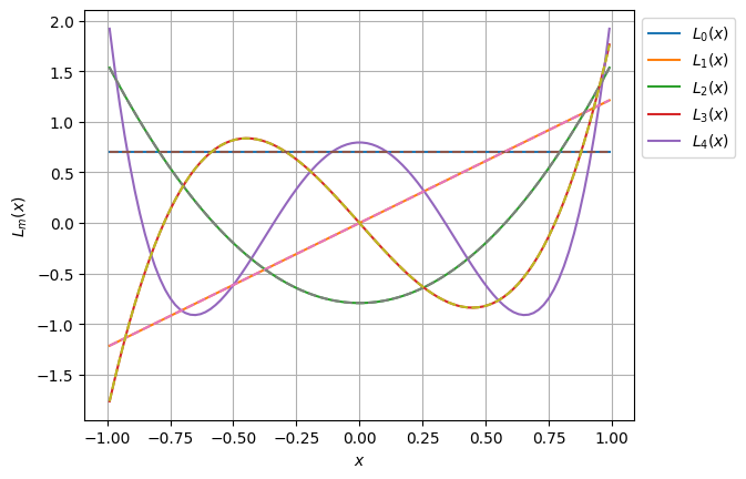
Check your results against the following numerical solutions. Note: the individual basis functions \(L_m(x)\) are unique up to a phase, so you may need to multiply your solution by a phase like \(-1\) to get it to agree with these numerical results prepared using the numerical QR Decomposition

%matplotlib inline
import numpy as np, matplotlib.pyplot as plt

Nx = 100
Np = 5
x = np.linspace(-1, 1, 2*Nx+1)[1:-1:2]
dx = 2/Nx
n = np.arange(Np)
M = x[:, None]**n[None, :] * np.sqrt(dx)
Q, R = np.linalg.qr(M)
Lx = np.linalg.solve(R.T, M.T).T/np.sqrt(dx)
Lx /= np.sign(Lx[-1, :])[None, :]
assert np.allclose(Lx.T.conj() @ Lx * dx, np.eye(Np))

fig, ax = plt.subplots()
for m in range(Np):
    ax.plot(x, Lx[:, m], '-', label=f"$L_{{{m}}}(x)$")

Ps = [[1], [1, 0], [1.5, 0, -0.5], [2.5, 0, -1.5, 0]]
for m in range(len(Ps)):
    ax.plot(x, np.polyval(Ps[m], x)/np.sqrt(2/(2*m+1)), "--")
    
ax.set(xlabel="$x$", ylabel="$L_m(x)$");
plt.grid('on')
ax.legend(bbox_to_anchor=(1,1), loc="upper left");