import mmf_setup;mmf_setup.nbinit()
import logging;logging.getLogger('matplotlib').setLevel(logging.CRITICAL)
%matplotlib inline
import numpy as np, matplotlib.pyplot as plt

$\newcommand{\vect}[1]{\mathbf{#1}} \newcommand{\uvect}[1]{\hat{#1}} \newcommand{\abs}[1]{\lvert#1\rvert} \newcommand{\norm}[1]{\lVert#1\rVert} \newcommand{\I}{\mathrm{i}} \newcommand{\ket}[1]{\left|#1\right\rangle} \newcommand{\bra}[1]{\left\langle#1\right|} \newcommand{\braket}[1]{\langle#1\rangle} \newcommand{\Braket}[1]{\left\langle#1\right\rangle} \newcommand{\op}[1]{\mathbf{#1}} \newcommand{\mat}[1]{\mathbf{#1}} \newcommand{\d}{\mathrm{d}} \newcommand{\D}[1]{\mathcal{D}[#1]\;} \newcommand{\pdiff}[3][]{\frac{\partial^{#1} #2}{\partial {#3}^{#1}}} \newcommand{\diff}[3][]{\frac{\d^{#1} #2}{\d {#3}^{#1}}} \newcommand{\ddiff}[3][]{\frac{\delta^{#1} #2}{\delta {#3}^{#1}}} \newcommand{\floor}[1]{\left\lfloor#1\right\rfloor} \newcommand{\ceil}[1]{\left\lceil#1\right\rceil} % The following allows KaTeX to render these for significantly improved % performance on CoCalc. \newcommand{\DeclareMathOperator}[2]{\newcommand{#1}{#2}} \DeclareMathOperator{\Tr}{Tr} \DeclareMathOperator{\erf}{erf} \DeclareMathOperator{\erfi}{erfi} \DeclareMathOperator{\sech}{sech} \DeclareMathOperator{\sn}{sn} \DeclareMathOperator{\cn}{cn} \DeclareMathOperator{\dn}{dn} \DeclareMathOperator{\sgn}{sgn} \DeclareMathOperator{\order}{O} \DeclareMathOperator{\diag}{diag} % \newcommand{\mylabel}[1]{\label{#1}\tag{#1}} \newcommand{\degree}{\circ}$

This cell adds /home/docs/checkouts/readthedocs.org/user_builds/physics-555-quantum-technologies/checkouts/latest/src to your path, and contains some definitions for equations and some CSS for styling the notebook. If things look a bit strange, please try the following:

• Choose "Trust Notebook" from the "File" menu.
• Re-execute this cell.
• Reload the notebook.

Landau-Zener Transitions

\(\newcommand{\sa}{\ket{\downarrow}}\newcommand{\sb}{\ket{\uparrow}}\)

The Landau-Zener formula for nonadiabatic transitions is a non-trivial example of the type of manipulation and level of mathematical sophistication expected in this course. This example serves several purposes. In particular, it:

1. contains the most general dynamics of a two-state system (qubit), providing a connection between dynamics on the Bloch Sphere and the analytic formulation of quantum mechanics.

2. represents the essence adiabatic quantum computing.

3. demonstrates a technique of analytically studying systems that are not analytically solvable.

General Qubit Dynamics

If the qubit is implemented as a spin-½ particle, then this corresponds to placing the particle in a time-dependent magnetic field

\[\begin{gather*} \vec{B}(t) = \frac{-2}{\hbar \mu_s}\vec{b}(t) \end{gather*}\]

where \(\mu_s\) is the spin magnetic dipole moment.

The most general dynamics for a single qubit can be described by the following Hamiltonian:

\[\begin{align*} \frac{\mat{H}(t)}{\hbar} &= \vec{b}(t) \cdot \vec{\mat{\sigma}} = b_x(t)\mat{\sigma_x} + b_y(t)\mat{\sigma_y} b_z(t)\mat{\sigma_z}\\ &= \begin{pmatrix} b_z(t) & b_x(t) - \I b_y(t)\\ b_x(t) + \I b_y(t) & -b_z(t) \end{pmatrix}. \end{align*}\]

The general dynamics of a qubit state \(\ket{\psi(t)}\) follow the time-dependent Schrödinger equation

\[\begin{gather*} \I\hbar \diff{}{t}\ket{\psi(t)} = \I\hbar \ket{\smash{\dot{\psi}}(t)} = \mat{H}(t)\ket{\psi(t)}. \end{gather*}\]

One will often see the following notation for the commutator of two matrices:

\[\begin{gather*} [\mat{A}, \mat{B}] = \mat{A}\mat{B} - \mat{B}\mat{A}. \end{gather*}\]

What makes this problem tricky (and quantum dynamics tricky in general) is that the matrices \(\mat{H}(t)\) at different times may not commute: i.e. there exists times \(t\) and \(t'\) such that

\[\begin{gather*} \mat{H}(t)\mat{H}(t') \neq \mat{H}(t')\mat{H}(t). \end{gather*}\]

Time Ordering: why it’s tricky.

If the Hamiltonian commutes at all times \([\mat{H}(t), \mat{H}(t')] = 0\) – e.g., if \(\mat{H}(t) = \mat{H}\) is constant – then the formal solution to the problem is simply:

\[\begin{gather*} \ket{\psi(t)} = \underbrace{ \exp\Biggl( \overbrace{\int_0^{t}\d{\tau}\; \frac{\op{H}(\tau)}{\I\hbar}}^{\mat{Q}(t)} \Biggr) }_{\mat{U}(t) = e^{\mat{Q}(t)}}\ket{\psi(0)}, \end{gather*}\]

where the unitary matrix \(\mat{U}(t)\) is the propagator. Recall from Matrix Exponential that this matrix exponential can be defined in terms of the Taylor series:

\[\begin{gather*} \mat{U}(t) = \mat{1} + \mat{Q}(t) + \frac{\mat{Q}^2(t)}{2!} + \cdots. \end{gather*}\]

Even in the second term, we see the problem:

\[\begin{gather*} \dot{\mat{Q}}(t) = \frac{\mat{H}(t)}{\I\hbar}, \\ \I \hbar \dot{\mat{U}}(t) = \op{H}(t) + \frac{\mat{H}(t)\mat{Q}(t) + \mat{Q}(t)\mat{H}(t)}{2} + \cdots. \end{gather*}\]

To recover the Schrödinger equation, we must pull all factors of \(\mat{H}(t)\) to the left so we have:

\[\begin{gather*} \I \hbar \dot{\mat{U}}(t) = \op{H}(t)\underbrace{ \Biggl( \mat{1} + \mat{Q}(t) + \frac{\mat{Q}^2(t)}{2!} + \cdots \Biggr)}_{\mat{U}(t)}, \end{gather*}\]

but we cannot do this if \(\mat{Q}(t)\) and \(\mat{H}(t)\) do not commute, which will generally be the case if the Hamiltonian does not commute at different times.

The solution is to work through this expansion, manually ordering all products of \(\mat{H}(t)\) so that later times appear to the left while earlier times appear to the left. This is done with the time ordering operator \(\mathcal{T}\):

\[\begin{gather*} \mathcal{T}\Bigl\{\mat{A}(t_a)\mat{B}(t_b)\Bigr\} = \begin{cases} \mat{A}(t_a)\mat{B}(t_b) & t_a > t_b\\ \mat{B}(t_b)\mat{A}(t_a) & t_a < t_b. \end{cases} \end{gather*}\]

Thus, once sometimes the solution written as

\[\begin{gather*} \mat{U}(t) = \mathcal{T}\left\{ \exp\Biggl( \int_0^{t}\d{\tau}\; \frac{\op{H}(\tau)}{\I\hbar} \Biggr) \right\}, \end{gather*}\]

but this does not really help solve the equation. Solving the differential equation numerically is usually the easiest approach, but this time-ordering can be useful when the time-dependence is perturbative.

Edwin Barns presents an interesting solution in [Barnes, 2013] that turns the problem around. Instead of specifying \(\vec{b}(t)\) and trying to find a solution, he shows that one can directly parameterize the propagator \(\mat{U}(t)\), then determine what magnetic field \(\vec{b}(t)\) gives this behavior.

Barns’s original presentation.

Barns introduces the functions \(β(t)\), \(φ(t)\), and \(χ(t)\), subject to the constraint

\[\begin{gather*} \abs{\dot{χ}(t)} < \abs{β(t)}, \\ χ(t) = 0, \qquad \dot{χ}(0) = -sβ(0). \end{gather*}\]

In the following expressions, we suppress the argument \(t\). All quantities except \(s = \pm 1\) are time-dependent:

\[\begin{gather*} \mat{U} = \begin{pmatrix} u_{11} & -u_{21}^*\\ u_{21} & u_{11}^* \end{pmatrix} = \begin{pmatrix} \vec{u} & -\I\mat{Y}\vec{u}^* \end{pmatrix},\\ \vec{u} = \begin{pmatrix} \cos(χ) e^{\I (ξ_{-} - φ/2)}\\ \I s \sin(χ) e^{\I (ξ_{+} + φ/2)} \end{pmatrix}, \\ ξ_{±} = \int_0^{t}β\sqrt{1-\frac{\dot{χ}^2}{β^2}}\csc(2χ)\d{\tau}\; \pm \frac{1}{2}\sin^{-1}\frac{\dot{χ}}{β} \pm s\frac{π}{4},\\ \vec{b} = \begin{pmatrix} β\cos φ\\ β\sin φ\\ \frac{\ddot{χ} - \dot{χ}\dot{β}/β}{2β\sqrt{1-\frac{\dot{χ}^2}{β^2}}} -β\sqrt{1-\frac{\dot{χ}^2}{β^2}}\cot(2χ) + \frac{\dot{φ}}{2} \end{pmatrix}. \end{gather*}\]

We replace \(\beta(t)\) with the angle \(\phi(t)\) where \(\cos \phi = \dot{\chi}/\beta\). This automatically satisfies the constraints if start with \(\phi(0) \in \{0, \pi\}\) (corresponding to \(s=-1\) and \(s=+1\) respectively):

\[\begin{gather*} \vec{u} = \I^{(1-s)/2} e^{\I\eta}\begin{pmatrix} \cos(χ)\\ -\I\sin(χ) e^{\I(φ + \phi)} \end{pmatrix}, \\ \eta = \int_0^{t}β\sin \phi\csc(2χ)\d{\tau}\; - \frac{\phi}{2},\\ \beta = \frac{\dot{χ}}{\cos\phi},\\ \vec{b} = \begin{pmatrix} β\cos φ\\ β\sin φ\\ -β\sin \phi \cot(2χ) + \frac{\dot{φ} - \dot{\phi}}{2} \end{pmatrix}. \end{gather*}\]

(This still needs the phases checked…)

#:tags: [hide-cell]

# Numerical checks of these equations
from scipy.integrate import solve_ivp

T = 5.0
hbar = 1

from phys_555_2022.utils import sigmas  # Pauli matrices

# "Random" functions
import sympy
t_, T_ = sympy.var('t_, T_')
beta_ = sympy.exp(2*t_ / T_) / T_
varphi_ = sympy.cos(2*np.pi * t_ / T_)**2 + 1
chi_ = (t_ / T_)


# Differentiate and make functions
get_beta, get_varphi, get_chi = [
    sympy.lambdify([t_, T_], 
                   [_x, _x.diff(t_), _x.diff(t_, t_)], 
                   "numpy") 
    for _x in (beta_, varphi_, chi_)]


def b(t, T=T):
    varphi, dvarphi, _ = get_varphi(t, T)
    chi, dchi, ddchi = get_chi(t, T)
    beta, dbeta, _ = get_beta(t, T)
    eta = np.sqrt(1 - (dchi/beta)**2)
    return [
      beta * np.cos(varphi),
      beta * np.sin(varphi),
      (ddchi - dchi*dbeta/beta) / 2 / beta / eta - beta*eta/np.tan(2*chi) + dvarphi/2,
      ]

def get_H(t):
    return np.einsum('i,iab->ab', b(t), sigmas)

def rhs(t, psi):
    dpsi = get_H(t) @ psi / 1j / hbar
    return dpsi

psi0 = np.array([1, 0j])
print(get_H(1e-5))
res = solve_ivp(rhs, t_span=(1e-5, T), y0=psi0)
t = res.t
res.y.shape
plt.plot(t, abs(res.y.T))

chi, dchi, ddchi = get_chi(t, T)
varphi, dvarphi, ddvarphi = get_varphi(t, T)
beta, dbeta, ddnbta = get_beta(t, T)
plt.plot(t, abs(np.cos(chi)), ':')
plt.plot(t, abs(np.sin(chi)), ':');

---------------------------------------------------------------------------
ModuleNotFoundError                       Traceback (most recent call last)
Cell In[2], line 9
      6 T = 5.0
      7 hbar = 1
----> 9 from phys_555_2022.utils import sigmas  # Pauli matrices
     11 # "Random" functions
     12 import sympy

ModuleNotFoundError: No module named 'phys_555_2022'

# New formulation
phi_ = sympy.acos(chi_.diff(t_)/beta_)

get_phi, = [
    sympy.lambdify([t_, T_], 
                   [_x, _x.diff(t_), _x.diff(t_, t_)], 
                   "numpy") 
    for _x in (phi_,)]

def bnew(t, T=T):
    varphi, dvarphi, _ = get_varphi(t, T)
    phi, dphi, _ = get_phi(t, T)
    chi, dchi, _ = get_chi(t, T)
    beta = dchi / np.cos(phi)
    return [
      beta * np.cos(varphi),
      beta * np.sin(varphi),
      -dchi * np.tan(phi)/np.tan(2*chi) + (dvarphi-dphi)/2,
      ]

ts = np.array([0.0001, 1.0])
np.allclose(b(ts), bnew(ts))

---------------------------------------------------------------------------
NameError                                 Traceback (most recent call last)
Cell In[3], line 2
      1 # New formulation
----> 2 phi_ = sympy.acos(chi_.diff(t_)/beta_)
      4 get_phi, = [
      5     sympy.lambdify([t_, T_], 
      6                    [_x, _x.diff(t_), _x.diff(t_, t_)], 
      7                    "numpy") 
      8     for _x in (phi_,)]
     10 def bnew(t, T=T):

NameError: name 'sympy' is not defined

#:tags: [hide-cell]

# Complete new solution
from scipy.integrate import solve_ivp

T = 5.0
hbar = 1

from phys_555_2022.utils import sigmas  # Pauli matrices

# "Random" functions
import sympy
t_, T_ = sympy.var('t_, T_')
varphi_ = sympy.cos(2*np.pi * t_ / T_)**2
chi_ = (t_ / T_)**2
phi_ = sympy.sin(2*np.pi * t_ / T_)


# Differentiate and make functions
get_phi, get_varphi, get_chi = [
    sympy.lambdify([t_, T_], 
                   [_x, _x.diff(t_)], 
                   "numpy") 
    for _x in (phi_, varphi_, chi_)]


def b(t, T=T):
    varphi, dvarphi = get_varphi(t, T)
    chi, dchi = get_chi(t, T)
    phi, dphi = get_phi(t, T)
    beta = dchi / np.cos(phi)
    return [
      beta * np.cos(varphi),
      beta * np.sin(varphi),
      -beta*np.sin(phi)/np.tan(2*chi) + (dvarphi-dphi)/2,
      ]

def get_H(t):
    return np.einsum('i,iab->ab', b(t), sigmas)

def rhs(t, psi):
    dpsi = get_H(t) @ psi / 1j / hbar
    return dpsi

psi0 = np.array([1, 0j])
print(get_H(1e-5))
res = solve_ivp(rhs, t_span=(1e-5, T), y0=psi0)
t = res.t
res.y.shape
plt.plot(t, abs(res.y.T))

chi, dchi = get_chi(t, T)
varphi, dvarphi = get_varphi(t, T)
phi, dphi = get_phi(t, T)
plt.plot(t, abs(np.cos(chi)), ':')
plt.plot(t, abs(np.sin(chi)), ':');

---------------------------------------------------------------------------
ModuleNotFoundError                       Traceback (most recent call last)
Cell In[4], line 9
      6 T = 5.0
      7 hbar = 1
----> 9 from phys_555_2022.utils import sigmas  # Pauli matrices
     11 # "Random" functions
     12 import sympy

ModuleNotFoundError: No module named 'phys_555_2022'

a = beta/dchi
da = dbeta/dchi - beta*ddchi/dchi**2
w = np.arctanh(1/a)
#plt.plot(t, a);
gamma = 1/np.sqrt(1-(dchi/beta)**2)
plt.plot(t, 1/((ddchi - dchi*dbeta/beta)/2/beta*gamma), '-');
plt.plot(t, -1/(da/2*np.sinh(w)/a), ':');
plt.plot(t, -1/(da/2/a/np.sqrt(a**2-1)), ':');
#plt.plot(t, -beta/gamma, '-');
#plt.plot(t, -dchi/np.sinh(w), ':');
#plt.plot(t, -dchi*a/np.cosh(w), ':');

---------------------------------------------------------------------------
NameError                                 Traceback (most recent call last)
Cell In[5], line 1
----> 1 a = beta/dchi
      2 da = dbeta/dchi - beta*ddchi/dchi**2
      3 w = np.arctanh(1/a)

NameError: name 'beta' is not defined

{code-cell} ipython3
#:tags: [hide-cell]

# Numerical checks of these equations
from scipy.integrate import solve_ivp

T = 1.0
hbar = 1

from phys_555_2022.utils import sigmas  # Pauli matrices

# "Random" functions
import sympy
t_, T_ = sympy.var('t_, T_')
w_ = 1+sympy.sin(2*np.pi * t_ / T_)**2
phi_ = sympy.cos(2*np.pi * t_ / T_)**2 + 1
chi_ = (t_ / T_)**2


# Differentiate and make functions
get_w, get_phi, get_chi = [
    sympy.lambdify([t_, T_], sympy.Array([_x, _x.diff(t_)]), "numpy") 
    for _x in (w_, phi_, chi_)]


def b(t, T=T):
    phi, dphi = get_phi(t, T)
    chi, dchi = get_chi(t, T)
    w, dw = get_w(t, T)
    beta = dchi / np.tanh(w)
    return [
      beta * np.cos(phi),
      beta * np.sin(phi),
      dw / 2 /np.cosh(w) - dchi/np.tan(2*chi)/np.sinh(w) + dphi/2,
      ]

def get_H(t):
    return np.einsum('i,iab->ab', b(t), sigmas)

def rhs(t, psi):
    dpsi = get_H(t) @ psi / 1j / hbar
    return dpsi

psi0 = np.array([1, 0j])
res = solve_ivp(rhs, t_span=(1e-10,T), y0=psi0)
t = res.t
res.y.shape
plt.plot(t, abs(res.y.T))

w, dw = get_w(t, T)
chi, dchi = get_chi(t, T)
phi, dphi = get_phi(t, T)
beta = dchi/np.tanh(w)
plt.plot(t, abs(np.cos(chi)), ':')
plt.plot(t, abs(np.sin(chi)), ':')

The Landau-Zener Formula

These energies \(E_n(\lambda)\) are sometimes called energy “bands”, especially if the parameter \(\lambda = k\) is a (quasi-)momentum in some electronic material.

The general idea is to consider the eigenstates of a Hamiltonian \(\op{H}(\lambda)\ket{n(\lambda)} = \ket{n(\lambda)}E_n(\lambda)\) that depends on some parameter \(\lambda(t)\) which varies in time. As two bands cross, say \(E_0(\lambda_*) \approx E_1(\lambda_*)\), the Landau-Zener formula gives the transition probability as

\[\begin{gather*} P \approx e^{-2\pi \Gamma}, \qquad \Gamma = \frac{\norm{\braket{0|\op{H}|1}}^2} {\hbar\left\lvert\pdiff{(E_0 - E_1)}{t}\right\rvert} \end{gather*}\]

where everything is evaluated at the transition \(\lambda(t) = \lambda_*\) when the levels approach. (This formula is exact if several assumptions are made: see Landau-Zener formula for a discussion.)

Error

The numerator is not correct!

Note that the transition probability can be suppressed (i.e. large \(\Gamma\)) by:

• Changing the system slowly: This is the adiabatic theorem that ensures that a system will remain in its instantaneous eigenstate if varied slowly enough.

Alternative Formulation: Induced Transition

An alternate formulation is to consider a time-dependent Hamiltonian of the form:

\[\begin{gather*} \op{H}(t) = \op{A} + \lambda(t)\op{B}, \qquad \lambda(t\rightarrow \pm \infty) = 0. \end{gather*}\]

The question is: what is the probability of a state remaining in an specified eigenstate \(\ket{0}\) of \(\op{A}\) (typically the ground state, hence our notation) far in the future? I.e., if we start the system in the state \(\ket{\psi} = \ket{0}\) at time \(t=-\infty\), what is:

Convince yourself that \(P(\infty)\) is well defined. Hint: how do we know that once \(\lambda(t) \rightarrow 0\), \(P(t)\) does not oscillate?

\[\begin{gather*} P(\infty) = \lim_{t\rightarrow \infty} \overbrace{\norm{\braket{0|\psi(t)}}^2}^{P(t)}. \end{gather*}\]

Here we will consider the two-state problem where \(\op{A}\) has two eigenstates \(\ket{0}\) and \(\ket{1}\) with energies \(E_0=-E\) and \(E_1=E\) respectively, and the time-dependence is expressed through a coupling term:

\[\begin{gather*} \op{H}(t) = \ket{1}E\bra{1} - \ket{0}E\bra{0} + \lambda(t)\Delta\frac{\ket{0}\bra{1} + \ket{1}\bra{0}}{2}. \end{gather*}\]

Expressed in the \(\{\ket{0}, \ket{1}\}\) basis, the Hamltonian has the following matrix elements:

\[\begin{gather*} \mat{H}(t) = \begin{pmatrix} -E & \lambda(t)\frac{\Delta}{2}\\ \lambda(t)\frac{\Delta}{2} & E \end{pmatrix} = \tfrac{\Delta}{2}\lambda(t)\mat{\sigma}_x - E\mat{\sigma}_z. \end{gather*}\]

Appealing to our previous formulation, this is implemented by magnetic field:

\[\begin{gather*} \vec{u} \propto \begin{pmatrix} \cos(χ)\\ -\I\sin(χ) e^{\I(φ + \phi)} \end{pmatrix}, \qquad \beta = \frac{\dot{χ}}{\cos\phi},\\ \vec{b} = \begin{pmatrix} β\cos φ \\ β\sin φ \\ -β\sin \phi \cot(2χ) + \frac{\dot{φ} - \dot{\phi}}{2} \end{pmatrix} = \begin{pmatrix} \lambda(t)\tfrac{\Delta}{2\hbar}\\ 0\\ E/\hbar \end{pmatrix}. \end{gather*}\]

Thus, we are free to choose functions \(\chi(t)\) and \(\phi(t)\) such that

\[\begin{gather*} \chi(-\infty) = 0, \qquad \dot{\chi}(\infty) = 0, \qquad \chi(\infty) = \sin^{-1}\sqrt{P(\infty)}. \end{gather*}\]

Hence,

\[\begin{gather*} \varphi(t) = 0, \qquad \beta(t) = \lambda(t)\tfrac{\Delta}{2\hbar},\\ -\lambda(t)\tfrac{\Delta}{2}\sin \phi \cot(2χ) - \frac{\dot{\phi}}{2} = E/\hbar. \end{gather*}\]

Suppose we would like the transition

Analytic Solutions

The general Landau-Zener problem is not analytically solvable, but we can use the results from [Barnes, 2013]:

\[\begin{gather*} \vec{u} \propto\begin{pmatrix} \cos(χ)\\ -\I\sin(χ) e^{\I(φ + \phi)} \end{pmatrix}, \\ \vec{b} = \begin{pmatrix} β\cos φ\\ β\sin φ\\ -β\sin \phi \cot(2χ) + \frac{\dot{φ} - \dot{\phi}}{2} \end{pmatrix} = \begin{pmatrix} \tfrac{\Delta}{2\hbar}\\ 0\\ \frac{E}{\hbar}\lambda(t) \end{pmatrix}, \end{gather*}\]

hence

\[\begin{gather*} \varphi(t) = 0, \qquad \beta(t) = \tfrac{\Delta}{2\hbar} = \frac{\dot{χ}(t)}{\cos\phi(t)}, \\ \phi(t) = \cos^{-1}\Bigl(\frac{2\hbar\dot{χ}(t)}{\Delta}\Bigr),\\ \tfrac{E}{\hbar}\lambda(t) = -\tfrac{\Delta}{2\hbar}\sin \phi(t) \cot\bigl(2χ(t)\bigr) - \frac{\dot{\phi}(t)}{2} \end{gather*}\]

Note that if we start in state \(\ket{0}\) at time \(t=0\) with \(\chi(0)=0\), then the transition probability at time \(t\) is \(P_1(t) = \sin^2\chi(t)\). How fast can we effect such a transition? Well, we must keep \(\abs{\cos(\phi)} \leq 1\), so we have the so-called quantum speed limit:

\[\begin{gather*} \abs{\dot{\chi}} \leq \frac{\abs{\Delta}}{2\hbar}. \end{gather*}\]

The fastest transition can be implemented with:

\[\begin{gather*} \chi(t) = \frac{\Delta}{2\hbar}t, \qquad \phi(t) = 0, \qquad \lambda(t) = 0, \end{gather*}\]

effecting a complete transition in time \(t = 2\hbar/\abs{\Delta}\). This should make intuitive sense: we just let the magnetic field \(b_x\) effect the rotation. Any interference from \(b_z\) will rotate the spin towards \(b_x\), reducing its efficiency.

For the Landau-Zener problem we have

\[\begin{gather*} \vec{b} = \begin{pmatrix} \frac{\Delta}{2}\\ 0\\ E\lambda(t) \end{pmatrix}, \qquad \varphi = 0, \qquad \beta = \frac{\Delta}{2}, \\ E\lambda(t) = \frac{\hbar^2\ddot{\theta}(t)}{\sqrt{\Delta^2-4\hbar^2\dot{\theta}^2(t)}} -\frac{\cot 2\theta(t)}{2}\sqrt{\Delta^2 - 4\hbar^2\dot{\theta}^2(t)}. \end{gather*}\]

Note that if we start in state \(\ket{1}\) at time \(t=0\), then the transition probability at time \(t\) is:

\[\begin{gather*} P(t) = \abs{s(t)}^2 = \sin^2 \theta(t). \end{gather*}\]

We, if we start with \(\theta(0) = 0\), we can thus effect a perfect conversion by taking \(\theta(t) = \pi/2\). Note, however, that we must keep

\[\begin{gather*} \abs{\dot\theta} < \frac{\abs{\Delta}}{2\hbar}, \qquad t > \frac{\pi \hbar}{\abs{\Delta}}. \end{gather*}\]

This is sometimes called the quantum speed limit.

Alternative Formulation

In the alternative formulation, we have

\[\begin{gather*} \vec{b} = \begin{pmatrix} \frac{\Delta}{2}\lambda(t)\\ 0\\ E \end{pmatrix}, \qquad \varphi = 0, \qquad \beta = \frac{\Delta}{2}\lambda(t), \\ \diff{}{t}\ln \lambda(t) = \frac{ \hbar^2\ddot{\theta}(t) - E\sqrt{\Delta^2-4\hbar^2\dot{\theta}^2(t)} + \frac{\cot 2\theta(t)}{2}(\Delta^2 - 4\hbar^2\dot{\theta}^2(t))}{\dot{\theta}}. \end{gather*}\]

If we let \(\epsilon(t) = \sqrt{\Delta^2-4\hbar^2\dot{\theta}^2(t)}\), then we have

\[\begin{gather*} \dot{\theta}(t) = \frac{\sqrt{\Delta^2 - \epsilon^2(t)}}{2\hbar},\\ \ddot{\theta}(t) = \frac{-\epsilon(t)\dot{\epsilon}(t)}{2\hbar\sqrt{\Delta^2 - \epsilon^2(t)}},\\ \frac{\ddot{\theta}(t)}{\dot{\theta}(t)} = \frac{-\epsilon(t)\dot{\epsilon}(t)}{\Delta^2 - \epsilon^2(t)},\\ \diff{}{t}\ln \lambda(t) = \frac{ \hbar^2\ddot{\theta}(t) - E\epsilon(t) + \frac{\cot 2\theta(t)}{2}\epsilon^2(t)}{\dot{\theta}}. \end{gather*}\]

The idea is as follows.

Consider a time-independent Hamiltonian \(\op{H}_0\) with two eigenstates \(\ket{0}\) and \(\ket{1}\) with energies \(E_0\) and \(E_1\) respectively. To this, we add a time-dependent piece which mixes these:

The model considers the dynamics of the following time-dependent Hamiltonian that couples two states as expressed in the \(\op{S}_z\) basis \(\{\sa, \sb\}\):

In the notation of Barnes:2012, \(\beta = \Delta/2\), \(\alpha = E \omega t^2\).

\[\begin{gather*} \op{H} = \begin{pmatrix} E \omega t & \frac{\Delta}{2}\\ \frac{\Delta}{2} & -E \omega t \end{pmatrix} = \frac{\Delta}{2}\mat{\sigma}_x + E \omega t\mat{\sigma}_z. \end{gather*}\]

The question is: if we start in the state \(\sb\) at time \(t \ll 0\), what is the probability that the system will eventually transition to the state \(\sa\) far in the future \(t\gg 0\)?

from scipy.integrate import solve_ivp
from functools import partial

def get_H(t, w, delta, E=1.0):
    return np.array([
        [E*w*t, delta/2],
        [delta/2, -E*w*t]])

wts = np.linspace(-3, 3)
hbar = 1.0
w = 1.0
delta = 1.0
E = 1.0
Es = [np.linalg.eigvalsh(get_H(_t, w=w, delta=delta, E=E))
      for _t in wts/w]

fig, ax = plt.subplots()
ax.plot(wts, Es)
ax.set(xlabel=r"$\omega t$", ylabel="$E_n/E$");

def dpsi_dt(t, psi, w):
    Hpsi = get_H(t, w, delta=delta, E=E) @ psi
    return Hpsi / (2j * hbar)

wT = 10.0
psi0 = np.array([1, 0]) + 0j

ws = [0.1, 0.5, 1.0, 5.0, 10.0]
for w in ws:
    res = solve_ivp(partial(dpsi_dt, w=w), t_span=[-wT/w, wT/w], y0=psi0, t_eval=wts/w)
    Es = np.array(
        [(psi.T.conj() @ get_H(t, w=w, delta=delta, E=E) @ psi).real
         for (t, psi) in zip(res.t, res.y.T)])
    ax.plot(res.t*w, Es/E, ls="--", 
            label="$\hbar\omega={:.1f}E$".format(hbar*w/E))
ax.legend();

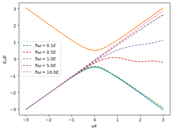
Our expectation is that, if the gap \(\Delta\) is large, and the rate of change is slow (large \(\tau\)), then we should remain in the ground state, otherwise we will transition.

Solution

We must solve the following differential equation

\[\begin{gather*} \I\hbar \ket{\dot{\psi}(t)} = \mat{H}(t)\ket{\psi(t)}, \qquad \ket{\psi(t\rightarrow - \infty)} = \begin{pmatrix} 1\\ 0\end{pmatrix} = \sb. \end{gather*}\]

References

• [Barnes, 2013]: An analytic reformulation of the problem that gives formulae for the magnetic field \(\vect{B}(t)\) required to effect transitions in the two-state system.

• [Jaffe, 2010]: A clean derivation of the classical Landau-Zener result using a semiclassical formalism that derives reflection probabilities using the duality between momentum and position.